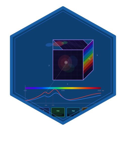

hyperspectR provides R workflows for hyperspectral research: file import, calibration, spectral processing, model fitting, inspection and reproducible exports. Version 0.3.0 produces research outputs; camera-specific and clinical accuracy require independent validation.
Installation
Requires R >= 4.1.0 and the required packages in DESCRIPTION, including viridisLite >= 0.4.0. From a local source checkout:
Rscript -e 'install.packages("remotes", repos = "https://cloud.r-project.org")'
Rscript -e 'remotes::install_local(".", dependencies = NA, upgrade = "never", build_vignettes = FALSE)'
These commands install required dependencies without updating unrelated packages. Update a dependency explicitly if an installed version is below its declared minimum. A source installation of compiled dependencies requires the platform’s R development toolchain. Building articles additionally requires knitr, rmarkdown and Pandoc. Optional readers and analysis backends are checked when their functions are called.
Quick Start
library(hyperspectR)

# Load example cube (synthetic 30x30 tissue scene, 61 bands, 430-910 nm)
cube <- hs_example_cube()
print(cube)

# Plot RGB composite
rgb <- ggplot2::autoplot(cube, type = "rgb")
rgb
ggplot2::ggsave("example-rgb.png", rgb, width = 7, height = 6)

# Fit the research hemoglobin fraction under the stated model
sto2 <- hs_sto2(cube)
hs_plot_index(sto2, title = "Fitted Hb fraction (%)", palette = "sto2")

# Research panel display; these are not vendor clinical indices
hs_plot_clinical(cube)
For the optional interactive explorer, install its runtime dependencies once, then launch it in an interactive R session:
install.packages(c("shiny", "bslib", "callr"), repos = "https://cloud.r-project.org")
hyperspectR::hs_run_app(hyperspectR::hs_example_cube())
The default example is synthetic. Recording uploads and background workers must fit available memory; max_upload_mb sets the upload limit in MiB.
Features
- I/O: Read ENVI, multi-channel TIFF, and Cubert .cu3s files
- Calibration: Dark correction, white reference normalization, bad pixel repair
- Preprocessing: Savitzky-Golay smoothing, SNV, MSC, spectral derivatives
- Research indices: fitted hemoglobin fraction, dimensionless band ratios and normalized differences
- Analysis: PCA, MNF, SAM classification, SVM/RF pixel classification, Beer-Lambert unmixing
- Visualization: ggplot2-based spectral plots, research panel displays, interactive Shiny app
- Research scope: Spectral measurements and model sensitivity; the supplied examples do not establish tissue oxygen saturation or diagnostic performance
Citation
To cite hyperspectR in publications, please use:
@Manual{,
  title = {hyperspectR: Hyperspectral Imaging Analysis for Biomedical Applications},
  author = {R. Heller and V. Forstmeier},
  year = {2026},
  note = {R package version 0.3.0},
  url = {https://github.com/cttir/hyperspectR},
}
Use the version actually analyzed and retain its source revision. This version has no confirmed published DOI; the prior identifier and observed publication state are retained in the maintenance record.
License
MIT; see the full license. The pinned hemoglobin reference data retain their upstream notice and provenance.
Corrected research semantics
The development version changes numerical behavior from 0.1.0. hs_sto2() now fits tabulated hemoglobin reference spectra; method = "ratio" raises a migration error. hs_band_ratio() and the legacy NPI/THI/TWI functions return dimensionless, unscaled ratios. They are not vendor clinical indices or calibrated physiological measurements. The simulator is a software demonstration, not validation data.
hs_beer_lambert() requires a declared reflectance/absorbance domain. It returns coefficients in mol/L * cm; concentrations is available only with a supplied pathlength_cm. Sensor response and tissue scattering require separate evaluation.
See the repository’s migration details, implementation record, and analysis protocol.
Reproducible processing
recipe <- hs_recipe(list(list(method = "smooth", args = list(window = 5))))
processed <- hs_process(hs_example_cube(), recipe)
# Use the saved recipe; MSC references, if present, are fitted only once.
new_data <- hs_process(hs_example_cube(), processed$recipe, learn = FALSE)
hs_batch() saves input checksums, recipes, results, implementation fingerprints and environment versions, isolates failed recordings, and resumes matching work. hs_grouped_evaluate() keeps subjects together across validation splits; hs_group_summary() reports uncertainty using independent groups rather than pixels.
Device readers are covered by software fixtures and SDK mocks. Real camera, phantom and independently labeled study validation remain separate evidence gates.
Use of LLM tools
Where applicable, LLM tools were used for narrowly defined, non-authorial tasks: copyediting, prose refinement, Markdown/LaTeX formatting, boilerplate scaffolding (such as CI configurations and build scripts), and code refactoring. Tools included Chat AI, the KISSKI (GWDG) service, and self-hosted Mistral Small (24B, Apache-2.0) served through a local vLLM architecture on an Ubuntu Linux workstation with Intel processors and NVIDIA GPUs. Self-hosted use also includes models that were further trained (fine-tuned) or weight-edited in-house for specific tasks. All self-hosted models ran locally, with no data sent to third parties.
All scientific claims, methodological choices, analyses, interpretations and conclusions remain the authors’ own. Where applicable, LLM-generated material must be reviewed and revised before inclusion, and references must be verified against their DOI, arXiv ID or ISBN.
Local software setup: vLLM with Python/PyTorch, plus R and RStudio.
Branding
Editable R sources and regeneration instructions are in tools/branding.