Compositions with inspectable spectral quantities • hyperspectaculR

The 0.2.0 candidate creates compositions and descriptive summaries from an hsi_cube or real numeric (rows, cols, bands) array. Reading recordings and calibration happen upstream. The default label is input value: a range such as 0–1 does not establish calibrated reflectance. These plots do not support physiological inference.

Inputs and missing observations

cube <- hsa_demo_cube(rows = 24, cols = 32, bands = 12, seed = 42)
cube$mask <- matrix(TRUE, 24, 32)
cube$mask[1:3, ] <- FALSE
cube$data[10, 10, 2] <- Inf
cube$data[11, 10, 3] <- NA_real_

A mask must be a logical spatial matrix without missing entries. FALSE excludes a pixel; nonfinite observations are excluded separately. Metadata must contain one strictly increasing finite wavelength in nm per band. Arrays can carry mask and wavelengths attributes. Without wavelengths the coordinates are band indices; physical selection and slopes require nm.

hsa_spectral_density(cube$data, nbins = 32)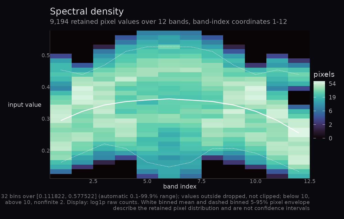

Selection and display domains

p <- hsa_mandala(cube, n_rings = 8, sampling = "wavelength")
p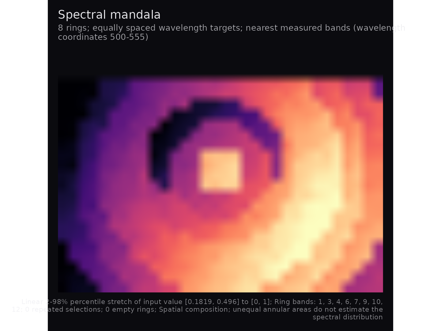

hsa_provenance(p)$selection$ring_band_indices
#> [1]  1  3  4  6  7  9 10 12

Default mandala targets are linear in band index. Physical targets are equally spaced in nm and select nearest measured bands, with ties toward shorter wavelengths. Repeated selections and empty rings preserve geometry; the full selection is in provenance. Unequal ring areas are a spatial composition, not a spectral distribution estimate. One ring selects the first band.

strict <- hsa_fusion(cube)
available <- hsa_fusion(cube, red = 9:12, green = 5:8, blue = 1:4,
                        missing = "available")
available
#> Warning: Removed 96 rows containing missing values or values outside the scale range
#> (`geom_raster()`).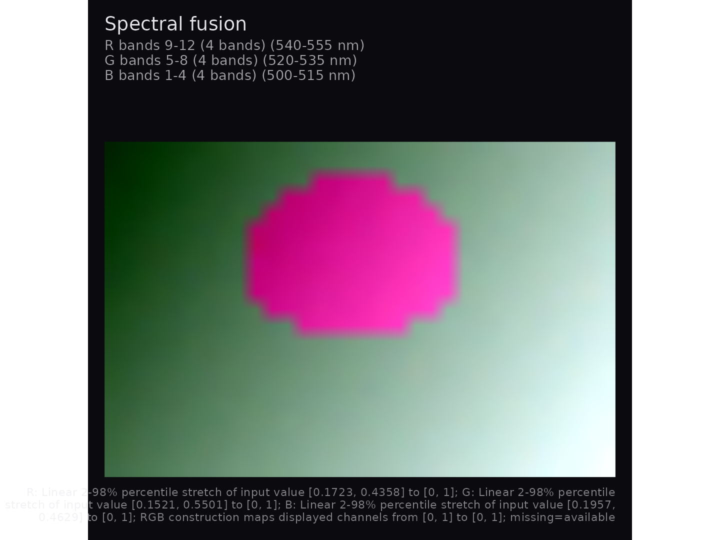

hsa_provenance(available)$missingness$contributors
#> $red
#> $red$selected_bands
#> [1] 4
#> 
#> $red$minimum
#> [1] 0
#> 
#> $red$maximum
#> [1] 4
#> 
#> $red$complete_pixels
#> [1] 672
#> 
#> $red$no_contributor_pixels
#> [1] 96
#> 
#> 
#> $green
#> $green$selected_bands
#> [1] 4
#> 
#> $green$minimum
#> [1] 0
#> 
#> $green$maximum
#> [1] 4
#> 
#> $green$complete_pixels
#> [1] 672
#> 
#> $green$no_contributor_pixels
#> [1] 96
#> 
#> 
#> $blue
#> $blue$selected_bands
#> [1] 4
#> 
#> $blue$minimum
#> [1] 0
#> 
#> $blue$maximum
#> [1] 4
#> 
#> $blue$complete_pixels
#> [1] 670
#> 
#> $blue$no_contributor_pixels
#> [1] 96

All default RGB groups are disjoint contiguous index thirds, high bands to red, even with by = "wavelength". Explicit groups must all be supplied. They may overlap between channels; duplicates within a group are errors. A one-band explicit fusion is supported. Wavelength targets must be in range and resolve to distinct bands within each group:

hsa_provenance(hsa_fusion(cube, red = c(545, 555), green = c(525, 535),
                          blue = c(500, 510), by = "wavelength"))$selection
#> $by
#> [1] "wavelength"
#> 
#> $default
#> [1] FALSE
#> 
#> $red
#> $red$requested
#> [1] 545 555
#> 
#> $red$indices
#> [1] 10 12
#> 
#> $red$coordinates
#> [1] 545 555
#> 
#> 
#> $green
#> $green$requested
#> [1] 525 535
#> 
#> $green$indices
#> [1] 6 8
#> 
#> $green$coordinates
#> [1] 525 535
#> 
#> 
#> $blue
#> $blue$requested
#> [1] 500 510
#> 
#> $blue$indices
#> [1] 1 3
#> 
#> $blue$coordinates
#> [1] 500 510

missing = "propagate" requires every selected band. "available" averages finite contributors separately by channel, still requiring all three channels to have a contribution. It changes the contributing population and records each channel’s selected-band count, minimum/maximum contributors, complete-pixel count and no-contributor-pixel count. Per-pixel contributor counts are not retained. Missing RGB values are transparent.

p <- hsa_mandala(cube, n_rings = 8, stretch = "none",
                 display_limits = c(-1, 1))
hsa_provenance(p)$enhancement
#> $limits
#> [1] -1  1
#> 
#> $requested_method
#> [1] "none"
#> 
#> $effective_method
#> [1] "none"
#> 
#> $fallback
#> NULL
#> 
#> $probs
#> [1] 0.02 0.98
#> 
#> $quantile_type
#> [1] 7
#> 
#> $clipped_below
#> [1] 0
#> 
#> $clipped_above
#> [1] 0
#> 
#> $finite_count
#> [1] 672
#> 
#> $excluded_count
#> [1] 96
#> 
#> $display_limits
#> [1] -1  1

Range and type-7 percentile stretches map to [0, 1]. A collapsed percentile interval falls back to the finite range; constants map to the dark endpoint. "none" preserves raw values and requires them to fit the fixed domain. The record includes requested/effective method, fallback, raw endpoints and clipping/exclusion counts. Plot data keep raw_value (or raw RGB channels).

changed <- p + ggplot2::labs(title = "Selected spatial scene") +
  ggplot2::theme(plot.title = ggplot2::element_text(size = 16))
identical(hsa_provenance(p), hsa_provenance(changed))
#> [1] TRUE

Provenance describes the original rendering. Ordinary theme/lab additions preserve it; arbitrary later plot edits are not recalculated. Inspect each component before patchwork composition. The accessor rejects a combined patchwork. Records contain no source cube or arbitrary input metadata.

Exact density populations

density <- hsa_spectral_density(cube, nbins = 32, limits = c(.1, .6),
                                normalise = "band", show_limits = TRUE)
density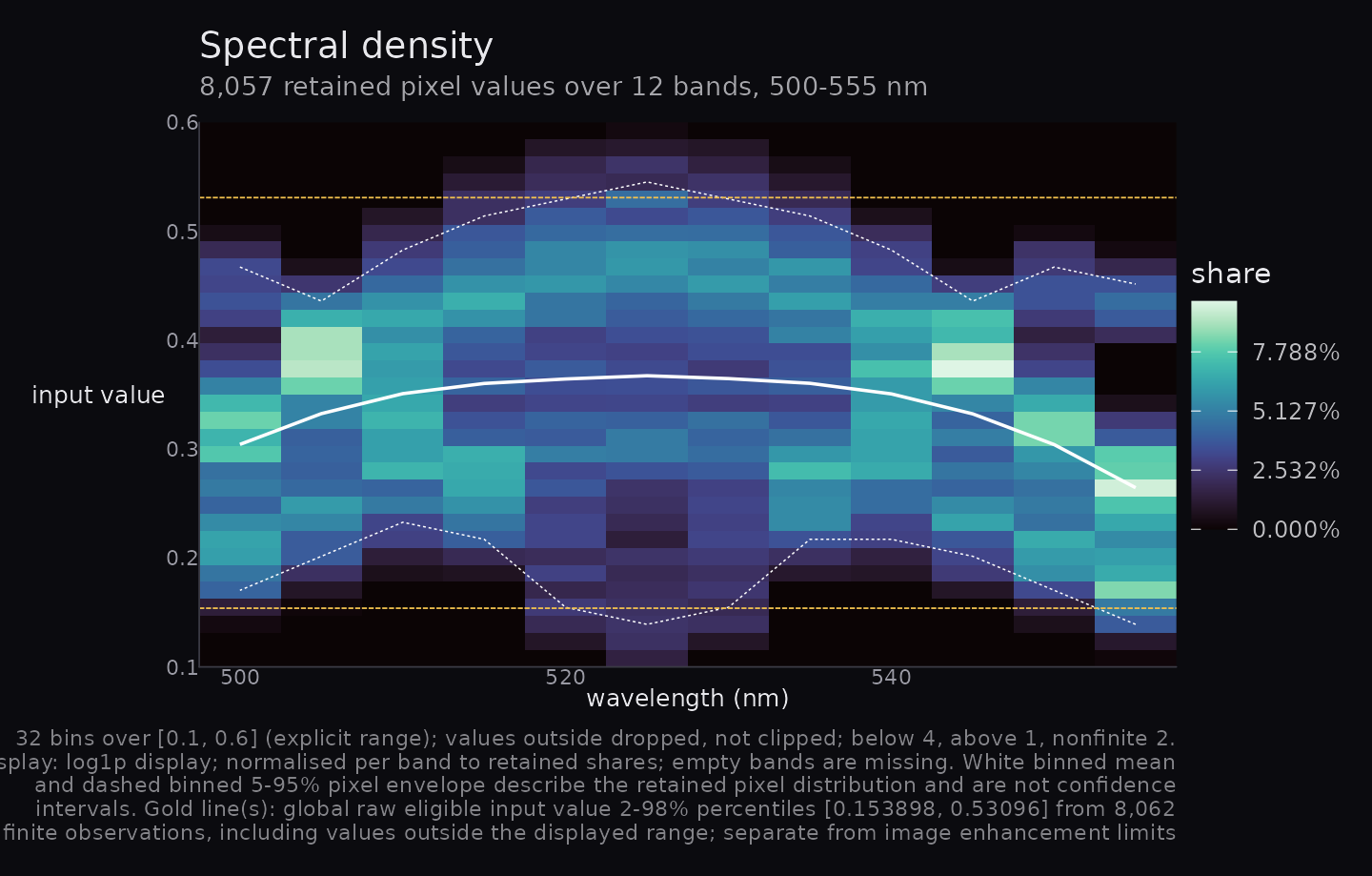

accounting <- hsa_provenance(density)$missingness
with(accounting, all(finite == below + kept + above))
#> [1] TRUE
with(accounting, all(eligible == finite + nonfinite))
#> [1] TRUE

Limits include both endpoints, with right-closed interior bins. Outside values are dropped, not clipped. Band shares divide by retained counts. Empty bands have missing shares and gaps in the overlays. White binned means and 5–95% pixel envelopes describe retained populations, not confidence intervals. Gold lines use global raw finite eligible observations, including those outside histogram limits; they are separate from image enhancement limits. Automatic limits use type-7 0.1–99.9% quantiles, with a disclosed finite-range or constant padding fallback. Irregular wavelengths have midpoint rectangle boundaries; single-band density discloses a width-one fallback. Raw H, breaks, references and accounting remain inspectable in the enhancement record.

Sampling and experimental summaries

For adjacent measured values, total variation is V = sum(abs(diff(x))); default mean step is V/(B-1) in input-value units per measured step. normalization = "wavelength_span" computes V/L in input value per nm. A rise from 0 to 1 across 400 nm has mean steps 0.5 and 0.2 at three and six samples, while both physical slopes equal 0.0025 per nm. Physical units define the quantity; they do not correct missing peaks, noise or unequal sampling.

example <- structure(list(data = array(c(0, 2, 2), c(1, 1, 3)),
                          wavelengths = c(500, 501, 505)), class = "hsi_cube")
hsa_spectral_flux(example, normalization = "wavelength_span")$data$raw_value
#> [1] 0.4
hsa_spectral_gradient(example)$data$raw_value
#> [1] 0.8944272
hsa_spectral_gradient(cube)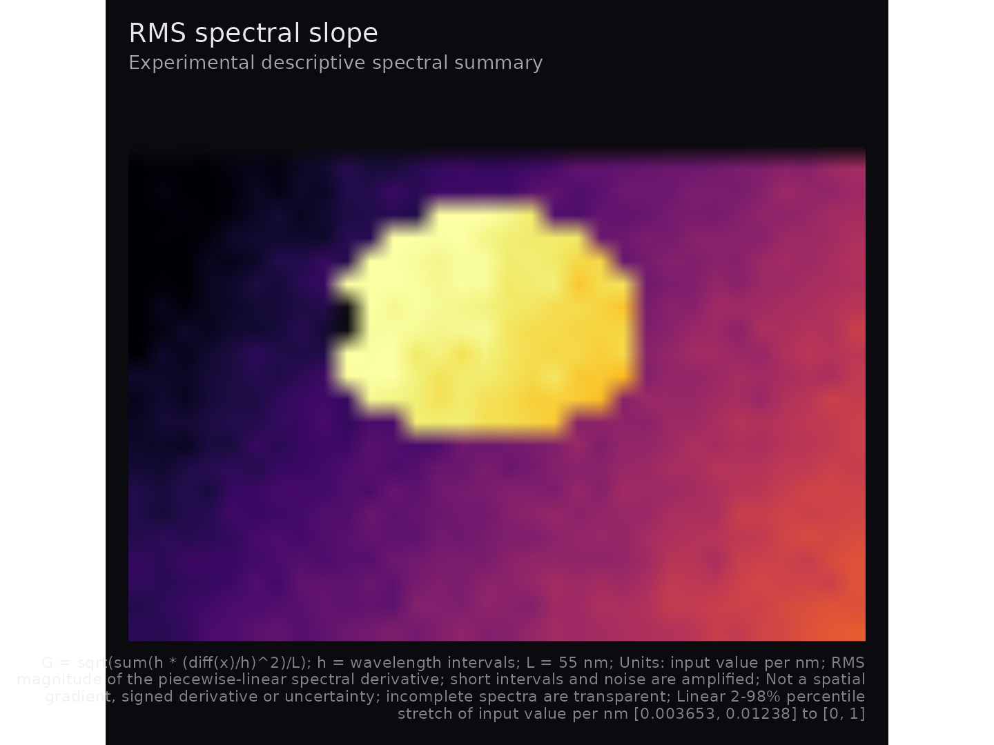

The independently verified values are 0.4 and approximately 0.894427 per nm. Experimental RMS slope is G = sqrt(sum(h * (diff(x)/h)^2)/L) for wavelength intervals h. It is nonnegative, loses derivative sign, and is not a spatial gradient or uncertainty. Short intervals amplify noise. On a flat signal with independent noise SD sigma, E[G^2] = 2 * sigma^2 / L * sum(1/h); increasing band count may increase this quantity. No smoothing or noise correction is applied. Both physical slopes bridge unobserved intervals with straight lines; interpolating extra points does not reconstruct absent information.

hsa_spectral_quartiles(cube)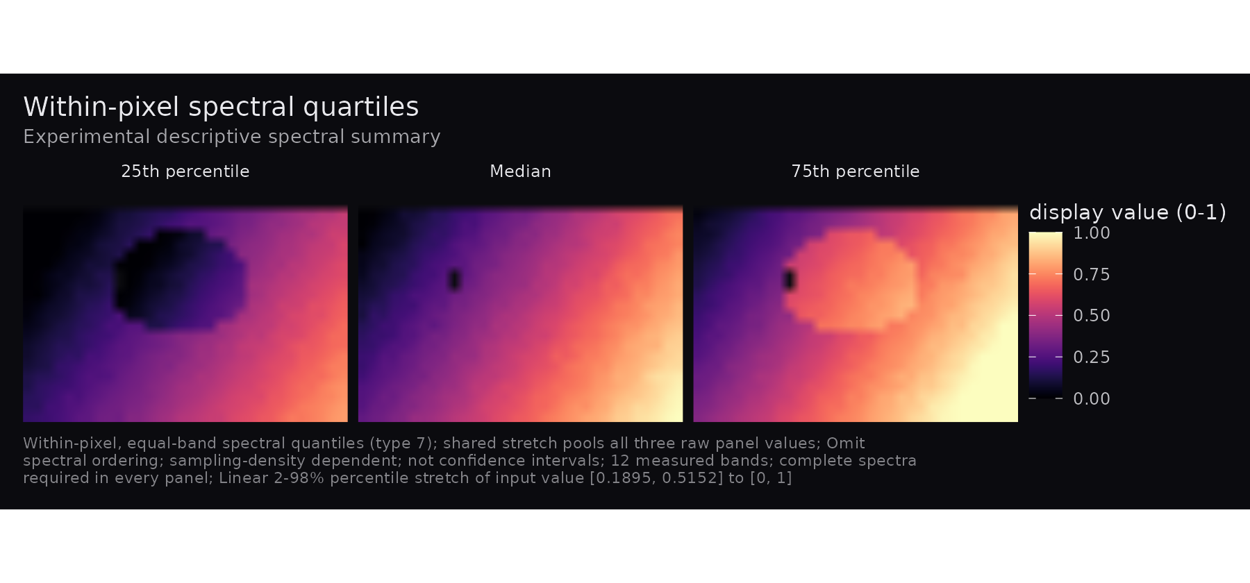

quartile_example <- array(c(0, 1, 4, 9), c(1, 1, 4))
hsa_spectral_quartiles(quartile_example)$data$raw_value
#> [1] 0.75 2.50 5.25

Type-7 quartiles are (0.75, 2.5, 5.25). Permuting the bands preserves them but can change flux. These experimental panels weight measured bands equally, discard order and depend on sampling density. They are not uncertainty intervals. All three panels share complete-spectrum validity and one pooled stretch/domain/legend. A single band gives identical panels. Experimental summaries offer descriptive comparisons, without universal instrument or sampling comparability.

Migration from 0.1.0

Masked/nonfinite pixels, dark endpoints, fusion thirds, raw domains, density geometry and retained counts can change visible output. Missing wavelengths are now labelled as indices. New exports include provenance, RMS slope and quartiles. Existing argument order and normalise remain supported; conflicting explicit normalise/normalization values error. Malformed metadata, fractional or out-of-range indices, duplicate within-group selections, incomplete RGB requests, invalid counts/probabilities and raw values outside the display domain now fail explicitly. Entirely invalid outputs fail instead of producing an apparently measured blank image.