Overview
phenoscapR provides tools for reading, processing, analysing, and visualising single-cell spatial biology data from multiplexed imaging platforms.
A typical workflow involves:
-
Reading cell segmentation data with
read_spatial() -
Quality control with
qc_filter() -
Normalisation with
normalise_markers() -
Phenotyping with
phenotype_cells() -
Spatial analysis with
nearest_neighbours(),cell_density(),interaction_matrix(), andspatial_clusters() -
Visualisation with
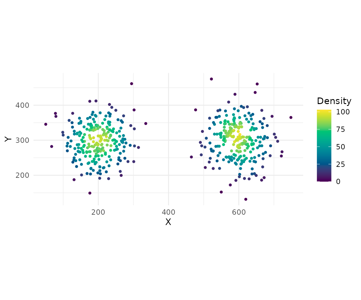
plot_cell_map(),plot_density(),plot_heatmap(), andplot_interactions()
Creating Example Data
Since real cell segmentation files can be large, we will create a small simulated data set for illustration.
library(phenoscapR)

set.seed(42)
n_cells <- 500

# Simulate two cell populations in different spatial regions
dt <- data.table::data.table(
  `Cell ID` = seq_len(n_cells),
  `Cell X Position` = c(rnorm(250, 200, 50), rnorm(250, 600, 50)),
  `Cell Y Position` = c(rnorm(250, 300, 50), rnorm(250, 300, 50)),
  `Cell Area (px)` = rlnorm(n_cells, log(100), 0.3),
  CD3 = c(rnorm(250, 800, 150), rnorm(250, 200, 100)),
  CD8 = c(rnorm(250, 200, 100), rnorm(250, 700, 120)),
  DAPI = rnorm(n_cells, 1000, 200)
)

# Write to a temporary CSV
tmp <- tempfile(fileext = ".csv")
write.csv(dt, tmp, row.names = FALSE)
Reading Data
cells <- read_spatial(tmp, sample_id = "example")
head(cells)
#>    sample_id cell_id        x        y cell_area      CD3         CD8      DAPI
#>       <char>   <int>    <num>    <num>     <num>    <num>       <num>     <num>
#> 1:   example       1 268.5479 351.4570 200.87599 709.7926 225.0578067 1123.4673
#> 2:   example       2 171.7651 345.7387 117.02725 779.6276 172.2075951  999.0918
#> 3:   example       3 218.1564 299.8772 133.80590 651.9091  27.5264266  981.7487
#> 4:   example       4 231.6431 306.8005 111.97350 924.7888  -0.6704944 1079.9919
#> 5:   example       5 220.2134 263.9923  74.17226 680.7411  70.8191670 1117.7803
#> 6: example 6 194.6938 290.0938 83.59012 851.0697 236.5838228 996.6244Normalisation
cells <- normalise_markers(cells, method = "zscore")
summary(cells[, c("CD3", "CD8", "DAPI")])
#>       CD3               CD8                DAPI
#>  Min.   :-1.6156   Min.   :-1.93580   Min.   :-2.97169
#>  1st Qu.:-0.9104   1st Qu.:-0.92825   1st Qu.:-0.63287
#>  Median :-0.2684   Median :-0.05788   Median : 0.05662
#>  Mean   : 0.0000   Mean   : 0.00000   Mean   : 0.00000
#>  3rd Qu.: 0.9048   3rd Qu.: 0.90400   3rd Qu.: 0.60278
#>  Max.   : 2.5022   Max.   : 2.39231   Max.   : 2.70425
Phenotyping
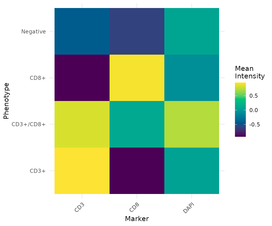
cells <- phenotype_cells(cells, thresholds = list(CD3 = 0, CD8 = 0))
summarise_phenotypes(cells)
Spatial Analysis
Nearest Neighbours
cells <- nearest_neighbours(cells, k = 5)
summary(cells$nn_distance)
#>    Min. 1st Qu.  Median    Mean 3rd Qu.    Max.
#>   4.794   7.516  10.435  13.540  15.533  89.053
Cell Density
cells <- cell_density(cells, radius = 50)
summary(cells$density)
#>    Min. 1st Qu.  Median    Mean 3rd Qu.    Max.
#>    0.00   33.00   55.00   53.76   77.00  103.00
Interaction Matrix
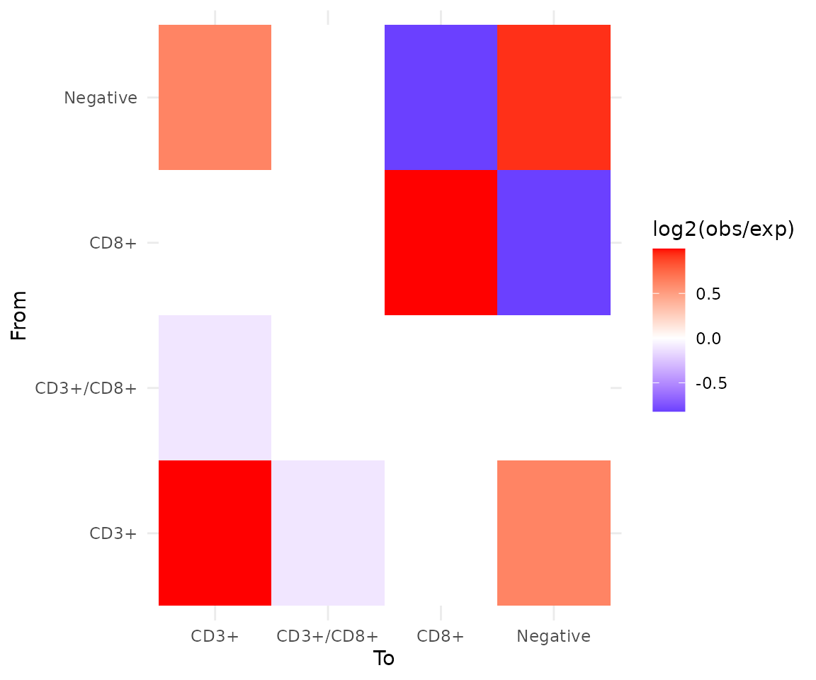
interactions <- interaction_matrix(cells, radius = 50)
interactions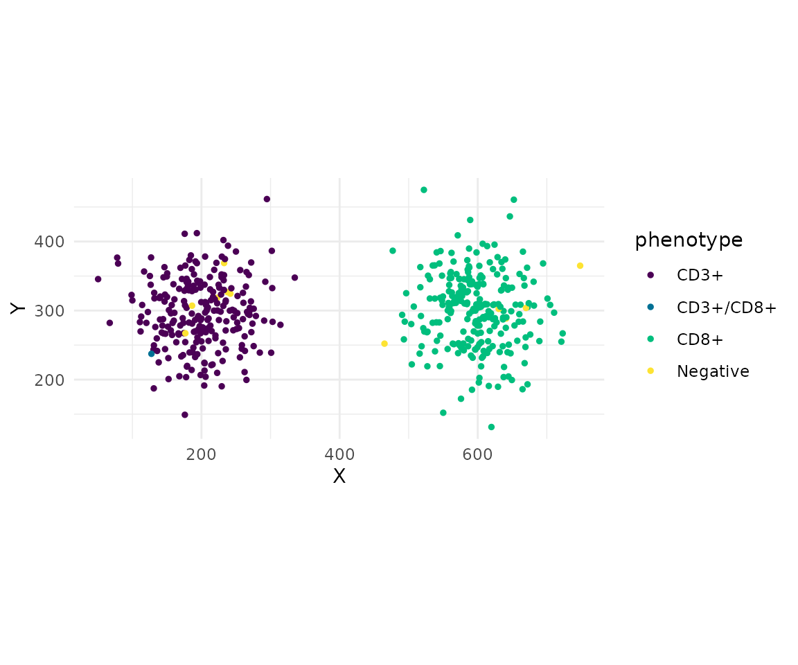
Use of LLM tools
Portions of this package were prepared with assistance from large
language model tooling for narrowly defined, non-authorial tasks:
copyediting, prose smoothing, Markdown/LaTeX formatting, scaffolding of
boilerplate files (CI configs, build scripts), code refactoring. The
tools used were Chat AI,
the LLM service of KISSKI (GWDG), and a self-hosted Mistral
Small (24B, Apache-2.0) run locally via Ollama and the ollamar R
package — local inference only, with no data sent to third parties for
the self-hosted model.
All scientific claims, methodological choices, analyses, interpretations, and conclusions are the author’s own. No LLM-generated text was incorporated without review and revision, and every reference was verified against its DOI, arXiv ID, or ISBN.