40 Case Study 3: Journal Portfolio Analysis
R. Heller · Date: 2026-05-09 · Last changed: 2026-10-31
40.1 Objective
Compare samples from three information-science journals using cumulative citation distributions, publication-cohort summaries, and assigned topics as a starting point for collection review.
40.3 Data acquisition
The source identifiers resolve to Scientometrics, Journal of Informetrics, and the Journal of the Association for Information Science and Technology (JASIST). These OpenAlex source records were checked on 2026-10-30. Historical titles of JASIST have separate source records and should not be substituted for this recent publication window.
journals <- tribble(
  ~short_name,        ~source_id,
  "Scientometrics",   "S148561398",
  "J. Informetrics",  "S205292342",
  "JASIST",           "S4210197613"
)
Request up to 300 randomly sampled articles per journal from 2018-2023, using a fixed seed. These samples do not measure the journals’ total output. The seed stabilises sampling within an OpenAlex snapshot; later database updates can change the returned records and citation counts. Preserve the returned works and cache files with any reported analysis.
fetch_journal <- function(sid) {
  works <- fetch_openalex(
    entity = "works",
    primary_location.source.id = sid,
    from_publication_date = "2018-01-01",
    to_publication_date = "2023-12-31",
    type = "article",
    options = list(sample = 300, seed = 42)
  )
  required <- c("id", "publication_year", "cited_by_count", "topics")
  if (!is.data.frame(works) || nrow(works) == 0L ||
      !all(required %in% names(works))) {
    stop("No usable journal sample returned for ", sid)
  }
  if (anyNA(works$id) || anyDuplicated(works$id) ||
      anyNA(works$publication_year) ||
      any(!works$publication_year %in% 2018:2023) ||
      any(!is.finite(works$cited_by_count)) || any(works$cited_by_count < 0)) {
    stop("Invalid or duplicate records in journal sample for ", sid)
  }
  works
}

journal_data <- journals |>
  mutate(works = map(source_id, fetch_journal))
40.4 Citation distributions in the samples
cited_by_count is the cumulative number of citations recorded when the data were retrieved, including citations received after 2023. It does not restrict citing papers to the sampled publication years. The h-index below describes only the returned sample, and all summaries remain unnormalised for field and publication year.
all_works <- journal_data |>
  mutate(works = map2(works, short_name, \(w, n) w |> mutate(journal = n))) |>
  pull(works) |>
  bind_rows()

ggplot(all_works, aes(x = journal, y = cited_by_count + 1)) +
  geom_boxplot(fill = palette_sci(1), alpha = 0.7) +
  scale_y_log10() +
  labs(x = NULL, y = "Cumulative citations + 1 (log10 scale)") +
  theme_sci()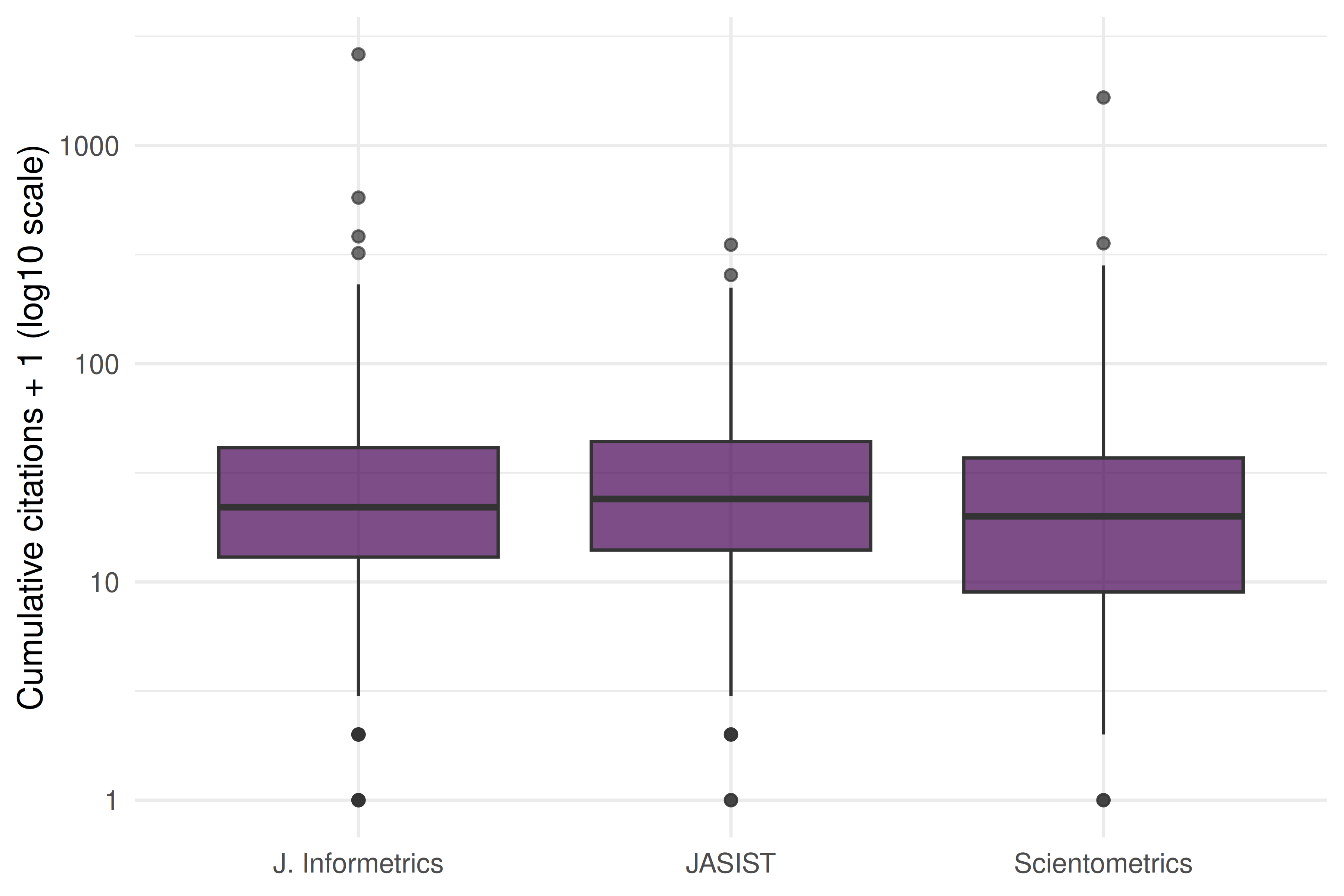
Figure 40.1: Cumulative citation distributions in the sampled articles, with one added before log scaling.
all_works |>
  group_by(journal) |>
  summarise(
    sampled_articles = n(),
    mean_cites = round(mean(cited_by_count), 1),
    median_cites = median(cited_by_count),
    sample_h_index = compute_h_index(cited_by_count),
    .groups = "drop"
  ) |>
  gt() |>
  cols_label(
    journal = "Journal", sampled_articles = "Sampled articles",
    mean_cites = "Mean cumulative citations", median_cites = "Median cumulative citations",
    sample_h_index = "Sample h-index"
)| Journal | Sampled articles | Mean cumulative citations | Median cumulative citations | Sample h-index |
|---|---|---|---|---|
| J. Informetrics | 300 | 45.4 | 21 | 54 |
| JASIST | 300 | 34.4 | 23 | 53 |
| Scientometrics | 300 | 37.1 | 19 | 51 |
40.5 Publication-cohort comparison
The following plot compares different publication cohorts at retrieval. Older cohorts have had more time to receive citations, and their composition may also differ. It is not a trajectory following the same articles over time, so it cannot establish citation-aging curves or citation half-lives. That requires time-resolved citation counts and an explicit observation window.
cohorts <- all_works |>
  group_by(journal, publication_year) |>
  summarise(mean_cites = mean(cited_by_count), sampled_articles = n(), .groups = "drop")

ggplot(cohorts, aes(x = publication_year, y = mean_cites, colour = journal)) +
  geom_line(linewidth = 1) +
  geom_point(aes(size = sampled_articles)) +
  scale_x_continuous(breaks = 2018:2023) +
  scale_colour_manual(values = palette_sci(3)) +
  labs(x = "Publication year", y = "Mean cumulative citations",
       colour = "Journal", size = "Sampled articles") +
  theme_sci()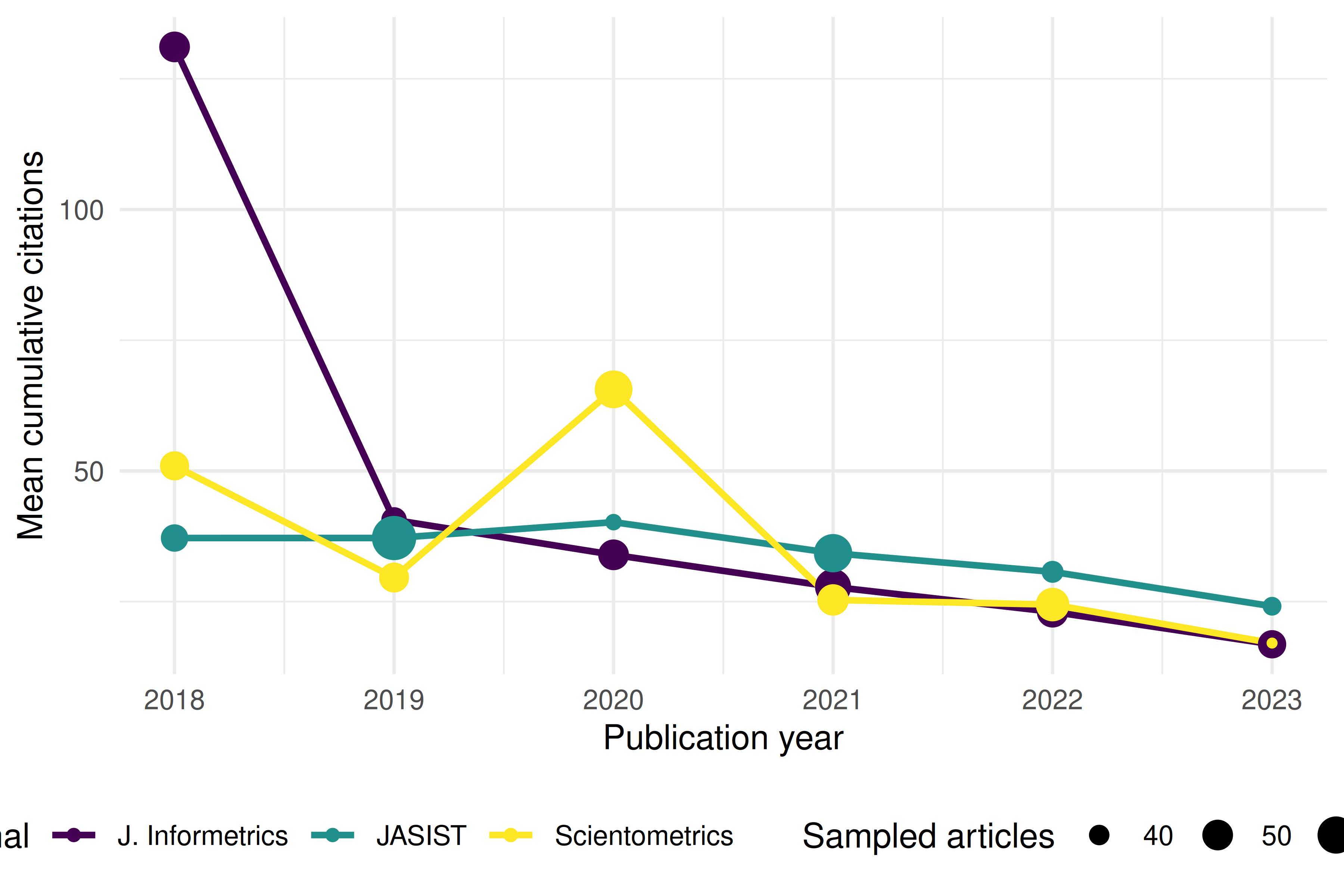
Figure 40.2: Mean cumulative citations by publication year in each journal sample; point size shows cohort sample size.
40.6 Topical coverage
Count each article once per assigned topic. The flattened topics table also contains the topics’ parent subfields, fields, and domains; retain only topic identifiers (T...). An article can contribute to several topics, while articles without topic assignments do not contribute to this chart; topic counts therefore need not sum to the number of sampled articles.
topic_data <- all_works |>
  select(id, journal, topics) |>
  unnest(topics, names_sep = "_") |>
  filter(str_detect(topics_id, "(^|/)T[0-9]+$")) |>
  select(id, journal, topic = topics_display_name) |>
  mutate(topic = str_to_lower(str_trim(topic))) |>
  filter(!is.na(topic), nchar(topic) >= 3) |>
  distinct(id, journal, topic)

top_topics <- topic_data |>
  count(journal, topic, sort = TRUE) |>
  group_by(journal) |>
  slice_max(n, n = 10, with_ties = FALSE) |>
  ungroup()
top_topics |>
  mutate(topic = reorder_within(topic, n, journal)) |>
  ggplot(aes(x = n, y = topic)) +
  geom_col(fill = palette_sci(1)) +
  facet_wrap(~ journal, scales = "free_y", ncol = 1) +
  scale_y_reordered() +
  labs(x = "Sampled articles assigned to topic", y = NULL) +
  theme_sci(base_size = 9)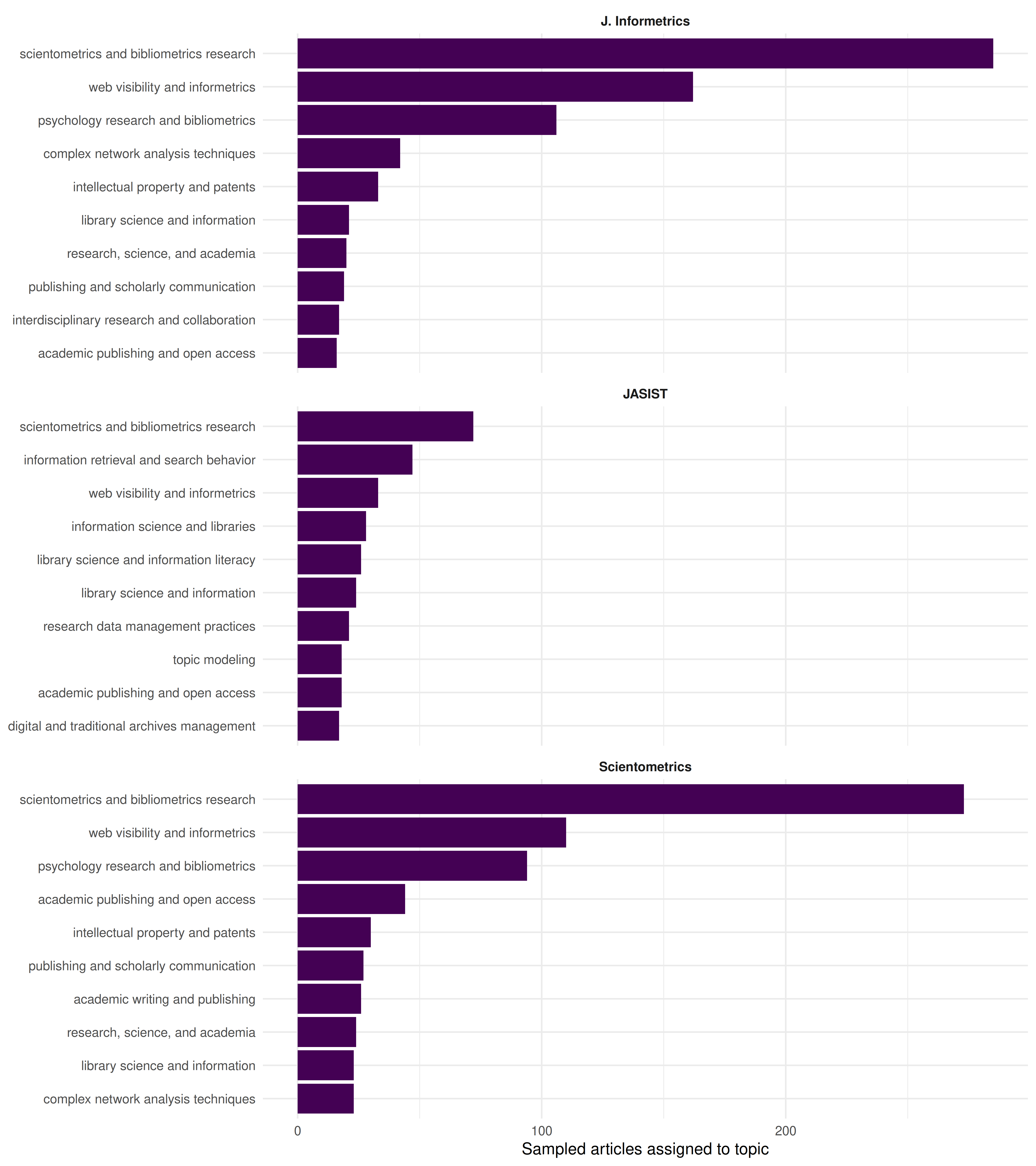
Figure 40.3: Up to 10 most frequent assigned topics in each journal sample.
40.7 Reading the results
- Citation distributions: Compare the plotted medians with the sample means. A large gap can indicate that a few highly cited articles dominate the mean; journal rankings should be reported only from the observed results.
- Publication cohorts: Compare cohorts alongside their sample sizes. Differences can reflect time available for citations, article composition, or sampling variation; they do not demonstrate a common aging curve.
- Assigned topics: Inspect overlap and differences in the displayed topics, then review representative articles before drawing conclusions about collection coverage.
40.8 Lessons learned
- Journal comparison requires multiple dimensions; no single metric tells the full story.
- Sample-based analysis is illustrative. Dependable journal evaluation requires a defined corpus, justified sampling or complete coverage, appropriate observation windows, and field-normalised indicators where relevant (Waltman 2016).
- Collection decisions also depend on local readership, access, cost, and subject needs; citation and topic summaries alone do not measure a journal’s value to a library.