33 Reproducibility, RRIDs, and Badges
R. Heller · Date: 2026-05-09 · Last changed: 2026-10-31
33.1 Learning objectives
After completing this chapter, you will be able to:
- Define reproducibility indicators and explain their role in research evaluation
- Search for data availability statements and open badges in bibliometric metadata
- Analyse the prevalence of reproducibility practices across journals and fields
- Discuss the relationship between transparency practices and citation impact
- Recognise the gap between reproducibility signalling and actual reproducibility
33.3 Conceptual background
The “replication crisis” has prompted widespread adoption of transparency practices: open data, open code, pre-registration, and registered reports. Bibliometrics can measure the uptake of these practices at scale, providing evidence for policy interventions.
Open badges are visual indicators (icons) attached to published papers that certify the availability of data, materials, or pre-registration. Journals like Psychological Science pioneered their use. Studies suggest that badges increase data sharing rates, though the quality of shared data varies.
Research Resource Identifiers (RRIDs) are persistent identifiers for research resources: antibodies, cell lines, model organisms, and software tools. Including RRIDs in methods sections improves reproducibility by enabling precise identification of the materials used. The RRID initiative has been adopted by over 1,000 journals.
Data availability statements (DAS) declare whether the data underlying a study are available and where to find them. Mandatory DAS policies have become common, but many statements say “data available upon request” without providing actual access. The presence of a DAS is easy to detect bibliometrically; the quality of actual data sharing is much harder to assess.
Code availability is increasingly expected, especially in computational fields. Journals like Nature require code availability statements. Platforms like GitHub, Zenodo, and Code Ocean facilitate code sharing, and DOIs for code repositories enable citation and tracking.
These practices are measurable proxies for reproducibility, but they are not reproducibility itself. A paper with an open badge may have unusable data; a paper without one may be perfectly reproducible. Hicks et al. (2015) warn against using transparency indicators as mechanical evaluation criteria.
33.4 Worked example
33.4.1 Analysing access status and metadata coverage
The example below measures article access status and abstract coverage in OpenAlex. It does not detect data/code availability, RRIDs, badges, or successful replication. Those questions require separate full-text/resource extraction and validation; OA status is not a validated substitute for them.
works <- fetch_openalex(
  entity = "works",
  primary_location.source.id = "S148561398",
  from_publication_date = "2018-01-01",
  to_publication_date = "2023-12-31",
  type = "article",
  options = list(sample = 400, seed = 42)
)

works_repro <- works |>
  transmute(
    id, display_name,
    year = year(publication_date),
    cited_by_count,
    oa_status,
    type,
    has_abstract = !is.na(abstract) & nzchar(trimws(abstract))
  )

cat(glue("Works: {nrow(works_repro)}\n"))
#> Works: 40033.4.2 Observed article access status
works_repro |>
  group_by(year) |>
  summarise(oa_rate = mean(oa_status != "closed", na.rm = TRUE),
            .groups = "drop") |>
  ggplot(aes(x = year, y = oa_rate)) +
  geom_line(linewidth = 1, colour = palette_sci(1)) +
  geom_point(size = 2, colour = palette_sci(1)) +
  scale_y_continuous(labels = scales::percent, limits = c(0, 1)) +
  labs(x = "Year", y = "OA rate") +
  theme_sci()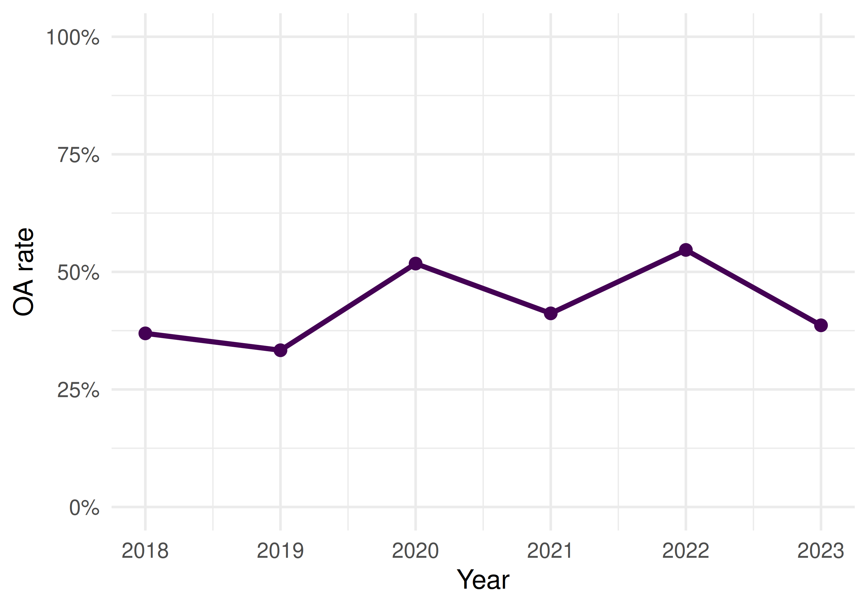
Figure 33.1: Open-access share among sampled articles with observed access status, by year.
33.4.3 Abstract availability as metadata completeness
works_repro |>
  group_by(year) |>
  summarise(abstract_rate = mean(has_abstract), .groups = "drop") |>
  ggplot(aes(x = year, y = abstract_rate)) +
  geom_line(linewidth = 1, colour = palette_sci(1)) +
  geom_point(size = 2, colour = palette_sci(1)) +
  scale_y_continuous(labels = scales::percent, limits = c(0, 1)) +
  labs(x = "Year", y = "Abstract available") +
  theme_sci()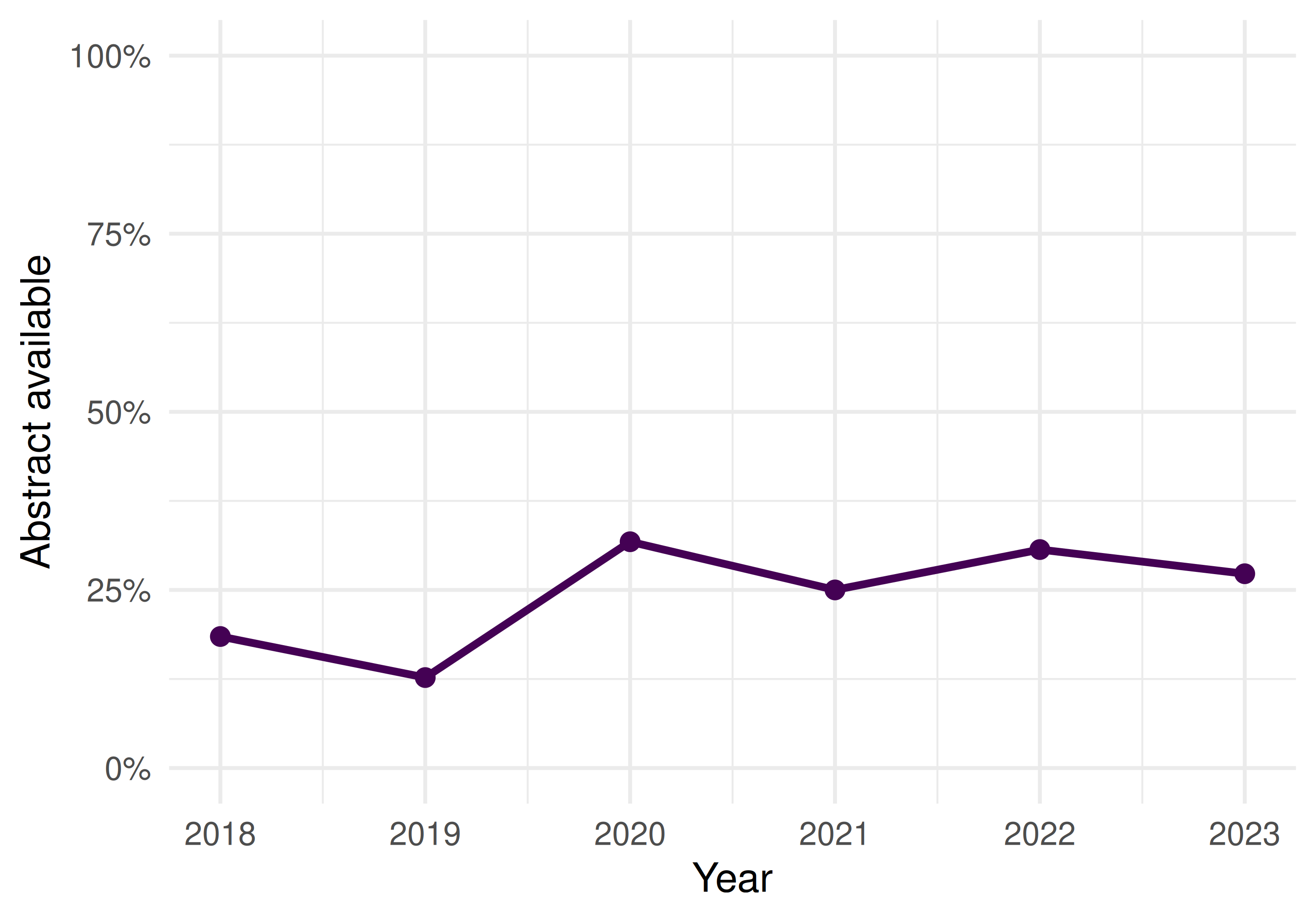
Figure 33.2: Abstract availability rate by year.
33.4.4 Access status and cumulative citations
works_repro |>
  mutate(is_oa = ifelse(oa_status != "closed", "OA", "Closed")) |>
  ggplot(aes(x = is_oa, y = cited_by_count + 1)) +
  geom_boxplot(fill = palette_sci(1), alpha = 0.7) +
  scale_y_log10() +
  labs(x = "Access status", y = "Citations (log scale)") +
  theme_sci()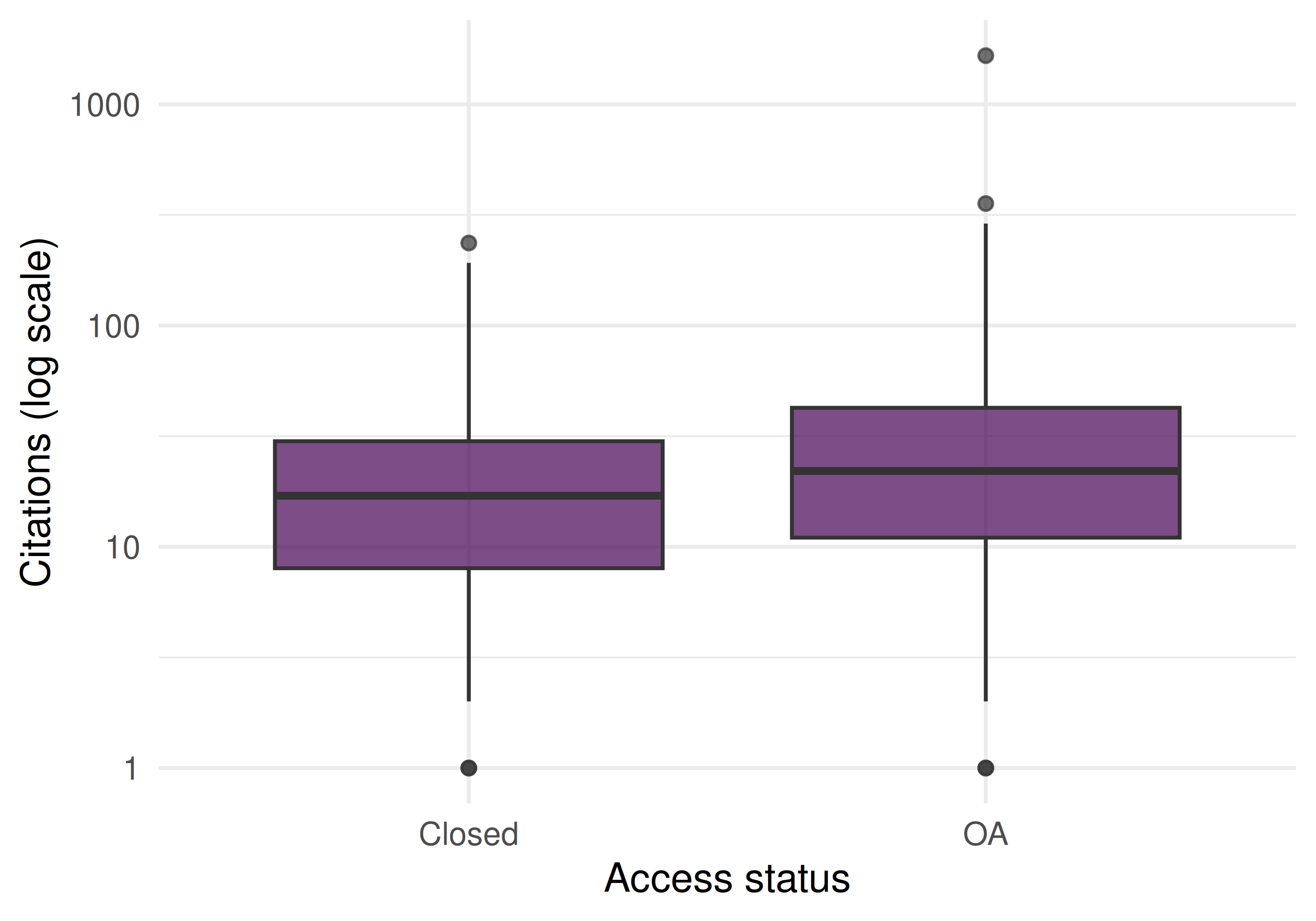
Figure 33.3: Current cumulative citation counts by recorded article access status.
33.4.5 Summary statistics
works_repro |>
  mutate(is_oa = oa_status != "closed") |>
  group_by(is_oa) |>
  summarise(
    n = n(),
    mean_cites = round(mean(cited_by_count), 1),
    abstract_rate = scales::percent(mean(has_abstract)),
    .groups = "drop"
  ) |>
gt()| is_oa | n | mean_cites | abstract_rate |
|---|---|---|---|
| FALSE | 225 | 24.2 | 0% |
| TRUE | 175 | 47.8 | 57% |
33.5 Diagnostics and interpretation
- Different constructs: Article access status and abstract coverage do not measure data/code sharing, RRID use, badge adoption or reproducibility. Check full texts and linked resources for those outcomes.
- Coverage over time: Changes in recorded access status or abstract coverage can reflect provider coverage and publication cohorts. The example does not evaluate a DAS or badge policy.
- Selection and exposure: Current cumulative citations mix publication ages, article selection and other confounders. The comparison cannot establish an OA effect or a relationship with open data.
- Field differences: Data sharing norms vary enormously. Genomics shares data routinely; clinical research often cannot due to privacy. Compare within fields.
33.7 Limitations and responsible use
- Signals are not substance. A data availability statement does not guarantee the data are actually available, usable, or correct. Badges certify process, not outcome.
- Mandates inflate compliance without improving practice. When journals require DAS, compliance rises but “available upon request” becomes the default, not genuine sharing.
- Reproducibility is multidimensional. No single indicator captures it. Data availability, code availability, methods transparency, pre-registration, and statistical rigour all contribute independently.
- Do not penalise fields where sharing is constrained. Clinical data (privacy), indigenous data (sovereignty), and sensitive social data cannot be freely shared. Mandating open data policies uniformly across fields is inappropriate (Hicks et al. 2015).
33.9 Common pitfalls
- Equating open data with reproducibility. Data can be open but undocumented, incorrectly formatted, or insufficient to reproduce the analysis.
- Counting badges without checking quality. A badge means the journal certified availability at publication time. The link may be broken or the data may have been removed.
- Ignoring negative results. Reproducibility also requires publishing null results and failed replications. These are poorly captured by current transparency indicators.
- Using transparency metrics as performance indicators. Transparency practices should be valued, but mechanically rewarding them creates perverse incentives (superficial compliance).
33.10 Exercises
DAS detection. For papers with full abstracts, search for keywords like “data availability”, “code availability”, or “github.com” in the abstract text. What proportion mention data or code sharing?
Cross-journal comparison. Compare abstract availability and OA rates for three journals. Do journals with higher OA rates also have better metadata completeness?
Temporal trends. Track recorded OA status and abstract coverage by publication cohort. Report the usable denominators and explain why these measures do not establish data/code sharing or reproducibility.
33.11 Solutions
Solutions are provided in E.
33.12 Further reading
- Hicks et al. (2015) — The Leiden Manifesto: responsible use of metrics, including transparency indicators.
- Priem et al. (2022) — OpenAlex metadata as a basis for reproducibility analysis.
- American Society for Cell Biology (2012) — DORA: assessment should consider research practices, not just outputs.
33.13 Session info
#> R version 4.6.1 (2026-06-24)
#> Platform: x86_64-pc-linux-gnu
#> Running under: Ubuntu 24.04.5 LTS
#>
#> Matrix products: default
#> BLAS:   /usr/lib/x86_64-linux-gnu/openblas-pthread/libblas.so.3
#> LAPACK: /usr/lib/x86_64-linux-gnu/openblas-pthread/libopenblasp-r0.3.26.so;  LAPACK version 3.12.0
#>
#> locale:
#>  [1] LC_CTYPE=C.UTF-8       LC_NUMERIC=C           LC_TIME=C.UTF-8
#>  [4] LC_COLLATE=C.UTF-8     LC_MONETARY=C.UTF-8    LC_MESSAGES=C.UTF-8
#>  [7] LC_PAPER=C.UTF-8       LC_NAME=C              LC_ADDRESS=C
#> [10] LC_TELEPHONE=C         LC_MEASUREMENT=C.UTF-8 LC_IDENTIFICATION=C
#>
#> time zone: UTC
#> tzcode source: system (glibc)
#>
#> attached base packages:
#> [1] stats     graphics  grDevices utils     datasets  methods   base
#>
#> other attached packages:
#>  [1] uwot_0.2.5                Matrix_1.7-5
#>  [3] word2vec_0.4.1            stm_1.3.10
#>  [5] topicmodels_0.2-17        quanteda.textstats_0.97.2
#>  [7] visNetwork_2.1.4          ggraph_2.2.2
#>  [9] tidygraph_1.3.1           igraph_2.3.4
#> [11] quanteda_4.5.1            pdftools_3.9.1
#> [13] arrow_26.0.1.1            bibliometrix_5.5.0
#> [15] RefManageR_1.4.0          bib2df_1.1.2.0
#> [17] rcrossref_1.2.1           gt_1.4.0
#> [19] tidytext_0.4.3            glue_1.8.1
#> [21] openalexR_3.1.2           lubridate_1.9.5
#> [23] forcats_1.0.1             stringr_1.6.0
#> [25] dplyr_1.2.1               purrr_1.2.2
#> [27] readr_2.2.0               tidyr_1.3.2
#> [29] tibble_3.3.1              ggplot2_4.0.4
#> [31] tidyverse_2.0.0
#>
#> loaded via a namespace (and not attached):
#>   [1] bibtex_0.5.3           RColorBrewer_1.1-3     rstudioapi_0.19.0
#>   [4] jsonlite_2.0.0         magrittr_2.0.5         modeltools_0.2-25
#>   [7] farver_2.1.2           rmarkdown_2.32         fs_2.1.0
#>  [10] vctrs_0.7.3            memoise_2.0.1          askpass_1.2.1
#>  [13] base64enc_0.1-6        htmltools_0.5.9        contentanalysis_1.1.1
#>  [16] curl_8.1.0             broom_1.0.13           janeaustenr_1.0.0
#>  [19] cellranger_1.1.0       sass_0.5.0             bslib_0.12.0
#>  [22] htmlwidgets_1.6.4      tokenizers_0.3.0       plyr_1.8.9
#>  [25] httr2_1.3.0            plotly_4.12.1          cachem_1.1.0
#>  [28] dimensionsR_0.0.3      mime_0.13              lifecycle_1.0.5
#>  [31] pkgconfig_2.0.3        R6_2.6.1               fastmap_1.2.0
#>  [34] shiny_1.15.0           digest_0.6.39          patchwork_1.3.2
#>  [37] shinycssloaders_1.1.0  rprojroot_2.1.1        RSpectra_0.16-2
#>  [40] SnowballC_0.7.1        labeling_0.4.3         urltools_1.7.3.1
#>  [43] timechange_0.4.0       mgcv_1.9-4             polyclip_1.10-7
#>  [46] httr_1.4.9             compiler_4.6.1         here_1.0.2
#>  [49] bit64_4.8.6            withr_3.0.3            backports_1.5.1
#>  [52] S7_1.0.0               viridis_0.6.5          ggforce_0.5.0
#>  [55] MASS_7.3-65            bibliometrixData_0.3.0 tools_4.6.1
#>  [58] otel_0.3.0             stopwords_2.3          zip_3.0.2
#>  [61] httpuv_1.6.17          rentrez_1.2.4          nlme_3.1-169
#>  [64] promises_1.5.0         grid_4.6.1             stringdist_0.9.17
#>  [67] reshape2_1.4.5         generics_0.1.4         gtable_0.3.6
#>  [70] tzdb_0.5.0             rscopus_0.9.0          ca_0.72
#>  [73] data.table_1.18.6.1    hms_1.1.4              xml2_1.6.0
#>  [76] utf8_1.2.6             ggrepel_0.9.8          pillar_1.11.1
#>  [79] nsyllable_1.0.1        vroom_1.7.1            later_1.4.8
#>  [82] splines_4.6.1          tweenr_2.0.3           lattice_0.22-9
#>  [85] FNN_1.1.4.1            bit_4.6.0              tidyselect_1.2.1
#>  [88] tm_0.7-20              miniUI_0.1.2           downlit_0.4.5
#>  [91] knitr_1.52             gridExtra_2.3.1        NLP_0.3-3
#>  [94] bookdown_0.48          stats4_4.6.1           crul_1.6.0
#>  [97] xfun_0.62              graphlayouts_1.2.5     matrixStats_1.5.0
#> [100] DT_0.34.0              humaniformat_0.6.0     stringi_1.8.9
#> [103] qpdf_1.4.1             yaml_2.3.12            evaluate_1.0.5
#> [106] httpcode_0.3.0         cli_3.6.6              xtable_1.8-8
#> [109] jquerylib_0.1.4        Rcpp_1.1.2             readxl_1.6.0
#> [112] triebeard_0.4.1        XML_3.99-0.25          parallel_4.6.1
#> [115] assertthat_0.2.1       pubmedR_1.1.0          slam_0.1-56
#> [118] viridisLite_0.4.3      scales_1.4.0           crayon_1.5.3
#> [121] openxlsx_4.2.9         rlang_1.3.0            fastmatch_1.1-8