32 Causal Inference in Scientometrics
R. Heller · Date: 2026-05-09 · Last changed: 2026-10-31
32.1 Learning objectives
After completing this chapter, you will be able to:
- Distinguish causal from correlational claims in bibliometric research
- Explain the intervention and outcome data required for difference-in-differences
- Compute descriptive OA-by-publication-cohort comparisons without assigning a causal interpretation
- Distinguish a within-year comparison from validated matching or a regression-discontinuity design
- Recognise the assumptions underlying causal inference in observational bibliometric data
32.3 Conceptual background
Bibliometrics is rich in correlations: OA papers are more cited than closed-access papers; funded research receives more citations; papers in prestigious journals are cited more. But correlation does not imply causation. The OA citation advantage may reflect self-selection (better papers are more likely to be made OA), not the causal effect of open access. Separating cause from confound is essential for evidence-based science policy.
Difference-in-differences (DiD) exploits policy changes as natural experiments. If a funder mandates OA starting in year T, papers from that funder before and after T serve as the treatment group, while papers from a similar funder without the mandate serve as the control. The causal effect is estimated as the difference in trends between treatment and control groups. The key assumption is parallel trends: absent the intervention, both groups would have followed the same trajectory.
Regression discontinuity design (RDD) applies when treatment is assigned by a threshold. For example, grants are funded above a score cutoff; papers are accepted above a review score threshold. Comparing outcomes just above and just below the threshold isolates the causal effect of the treatment, under the assumption that units near the threshold are comparable.
Matching methods create comparable groups from observational data. Propensity score matching pairs treated units (e.g., OA papers) with control units (closed-access papers) that have similar observable characteristics (field, journal, year, team size). This reduces confounding but cannot eliminate unmeasured confounders.
All three methods require strong assumptions. In bibliometrics, violations are common: the parallel trends assumption may fail because of concurrent policy changes; the RDD threshold may be manipulable; matching cannot address unmeasured confounders like paper quality. Hicks et al. (2015) emphasise that quantitative analysis, however sophisticated, cannot replace expert judgement in research evaluation.
32.4 Worked example
32.4.1 A descriptive OA-by-publication-cohort comparison
This example samples papers from one journal and compares their current cumulative citation counts. The 2020 split is an arbitrary publication-cohort boundary, not a documented intervention. OA status is observed at retrieval, not recorded treatment assignment. Different publication years contain different papers with different citation exposure. Consequently, neither the interaction regression nor the cohort plot identifies a policy effect or tests a DiD parallel-trends assumption. DiD requires a defensible intervention, comparison design and outcome histories; see Callaway and Sant’Anna (2021).
The sample and citation snapshot describe the fetched data only; they are not journal totals or a frozen historical citation panel.
works <- fetch_openalex(
  entity = "works",
  primary_location.source.id = "S148561398",
  from_publication_date = "2016-01-01",
  to_publication_date = "2023-12-31",
  type = "article",
  options = list(sample = 500, seed = 42)
)

cohort_data <- works |>
  transmute(
    id, year = year(publication_date),
    cited_by_count,
    is_oa = case_when(
      oa_status %in% c("gold", "green", "hybrid", "bronze", "diamond") ~ TRUE,
      oa_status == "closed" ~ FALSE,
      TRUE ~ NA
    ),
    recent_cohort = year >= 2020,
    referenced_works_count
  )

excluded_records <- sum(!complete.cases(cohort_data))
cohort_data <- cohort_data |> drop_na()
stopifnot(!anyDuplicated(cohort_data$id), nrow(cohort_data) > 0)
cat(glue("Excluded incomplete records: {excluded_records}\n"))
#> Excluded incomplete records: 0#> Sampled complete records: 500#> OA: 210, Closed: 29032.4.2 Descriptive comparison
cohort_summary <- cohort_data |>
  group_by(is_oa, recent_cohort) |>
  summarise(mean_cites = mean(cited_by_count), n = n(), .groups = "drop") |>
  mutate(period = ifelse(recent_cohort, "2020-2023", "2016-2019"),
         group = ifelse(is_oa, "Open access", "Closed"))

ggplot(cohort_summary, aes(x = period, y = mean_cites, fill = group)) +
  geom_col(position = "dodge") +
  scale_fill_manual(values = palette_sci(2)) +
  labs(x = "Publication cohort", y = "Mean cumulative citations at retrieval", fill = "Access") +
  theme_sci()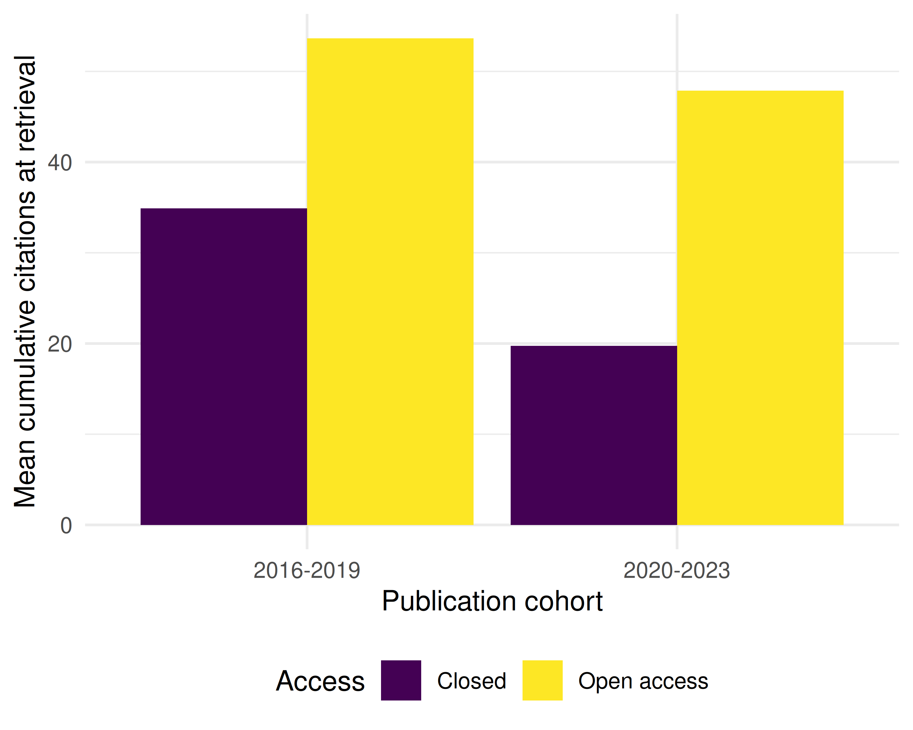
Figure 32.1: Current cumulative citations in sampled papers, grouped by OA status and publication cohort; not a policy-effect estimate.
32.4.3 Descriptive interaction regression
The interaction describes how the conditional OA/closed citation difference varies between the two sampled publication cohorts. Adding reference count is statistical adjustment, not an identification strategy. The fitted coefficients and conventional linear-model uncertainty summaries must not be reported as causal effects.
interaction_model <- lm(cited_by_count ~ is_oa * recent_cohort + referenced_works_count,
                data = cohort_data)

tidy_interaction <- broom::tidy(interaction_model)
tidy_interaction |>
  mutate(across(where(is.numeric), \(x) round(x, 3))) |>
gt()| term | estimate | std.error | statistic | p.value |
|---|---|---|---|---|
| (Intercept) | 21.53 | 8.661 | 2.486 | 0.013 |
| is_oaTRUE | 19.36 | 11.010 | 1.758 | 0.079 |
| recent_cohortTRUE | -18.30 | 9.880 | -1.852 | 0.065 |
| referenced_works_count | 0.30 | 0.124 | 2.415 | 0.016 |
| is_oaTRUE:recent_cohortTRUE | 9.64 | 15.179 | 0.635 | 0.526 |
32.4.4 Within-year sampling comparison
For each sampled OA paper, select one closed-access paper from the same publication year. Controls can be reused, and OA papers in years with no closed-access candidate are omitted. This is sampling with replacement within year, not propensity-score matching; it does not establish covariate balance or remove confounding.
oa_papers <- cohort_data |> filter(is_oa)
closed_papers <- cohort_data |> filter(!is_oa)

matched <- oa_papers |>
  mutate(match_year = year) |>
  inner_join(
    closed_papers |> select(year, control_id = id, cited_by_count_closed = cited_by_count),
    by = "year",
    relationship = "many-to-many"
  ) |>
  group_by(id) |>
  slice_sample(n = 1) |>
  ungroup()

cat(glue("Within-year pairs: {nrow(matched)} / {nrow(oa_papers)} OA papers\n"))
#> Within-year pairs: 210 / 210 OA papers#> Distinct closed-access controls: 142#> Mean cites (OA): 50.3#> Mean cites (closed match): 25.832.4.5 Publication-cohort profile
The horizontal axis is publication year. Each point summarises different papers’ cumulative citations at one retrieval time. These are not citations received annually by fixed treated and control groups.
trends <- cohort_data |>
  group_by(year, is_oa) |>
  summarise(mean_cites = mean(cited_by_count), .groups = "drop") |>
  mutate(group = ifelse(is_oa, "OA", "Closed"))

ggplot(trends, aes(x = year, y = mean_cites, colour = group)) +
  geom_line(linewidth = 1) +
  geom_point(size = 2) +
  geom_vline(xintercept = 2019.5, linetype = "dashed", colour = "grey50") +
  scale_colour_manual(values = palette_sci(2)) +
  labs(x = "Publication year", y = "Mean cumulative citations at retrieval", colour = "Access") +
  theme_sci()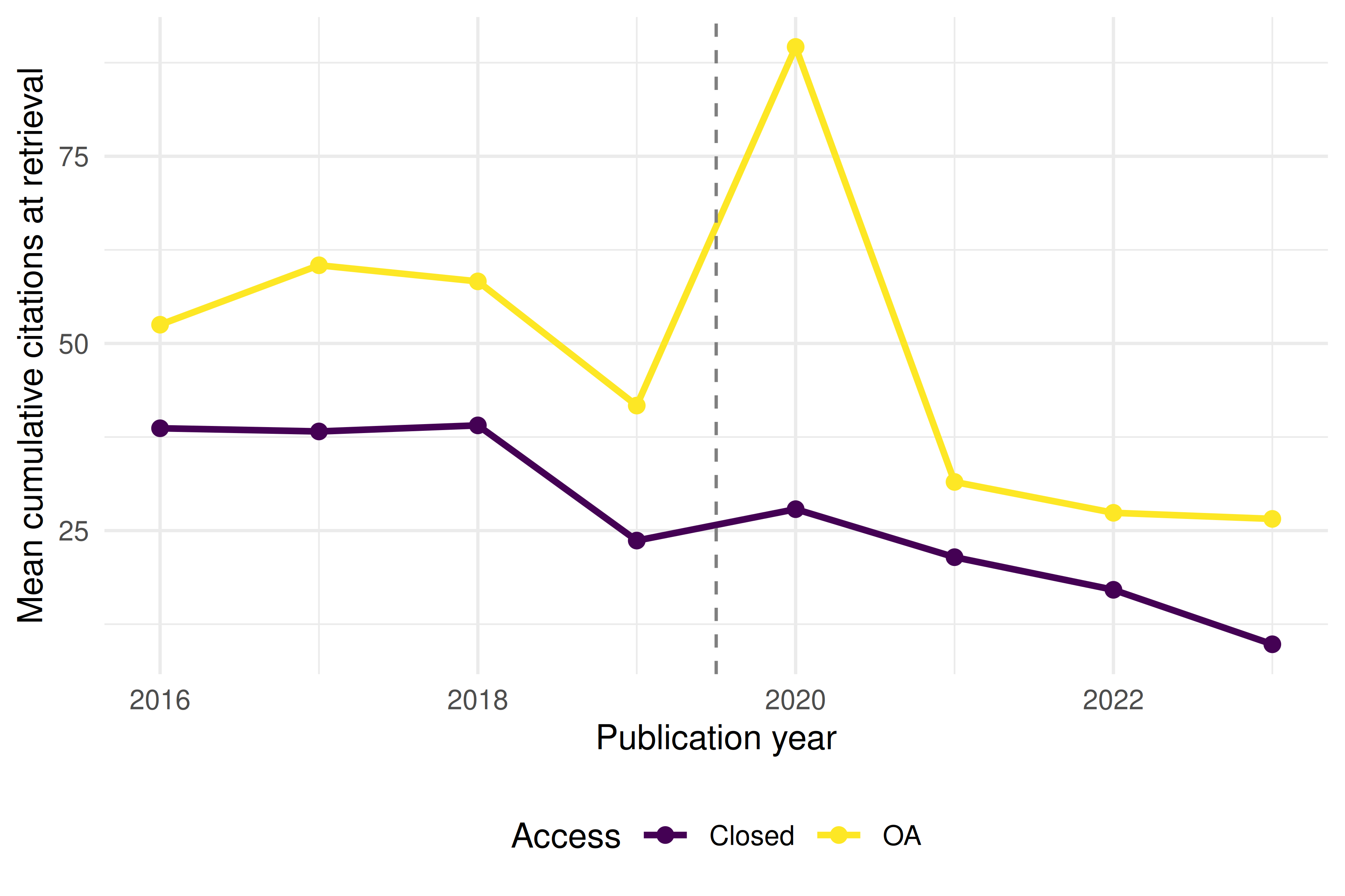
Figure 32.2: Current cumulative citations by OA status and publication year in the sample. This cohort profile does not test parallel trends.
32.5 Diagnostics and interpretation
- Selection and exposure: Report the sampling query, retrieval date, exclusions and group sizes. Older publication cohorts have longer citation exposure; snapshot OA status may differ from status at publication.
- Interpret the actual model: The OA-by-cohort coefficient is a descriptive conditional association. The arbitrary 2020 boundary supplies no intervention and no causal estimand.
- Assess the comparison: Check years without eligible controls, control reuse and covariate differences. One sampled same-year control does not make papers exchangeable.
- Causal designs need additional evidence: Define intervention timing and assignment, comparable outcomes over time, the target effect and identifying assumptions before choosing a DiD, RDD or matching analysis. A non-significant pre-trend test alone does not establish parallel counterfactual trends.
32.7 Limitations and responsible use
- This example is descriptive. It has no documented intervention or identified causal design. Observational causal designs can support causal interpretation under explicit, defensible assumptions; fitting the shown regression does not supply them.
- Unmeasured confounders. Paper quality, author reputation, and marketing effort are rarely observable in bibliometric data but strongly affect citations.
- Treatment definition. “OA” is not a single treatment — it encompasses gold, green, hybrid, and bronze, each with different mechanisms.
- Generalisability. This sampled single-journal comparison does not establish an OA effect in this journal or elsewhere.
- Policy implications require judgement. Even a well-estimated causal effect is one input into policy decisions, not a sufficient basis for mandates (Hicks et al. 2015; American Society for Cell Biology 2012).
32.9 Common pitfalls
- Claiming causation from regression coefficients. A positive OA coefficient in a regression does not prove OA causes more citations without addressing confounders.
- Calling a cohort profile a pre-trend test. Current cumulative citations in different publication cohorts do not measure treated/control outcome paths around a policy change.
- Treating matching as automatic identification. Choose covariates from the causal question and timing, evaluate overlap/balance, and avoid conditioning indiscriminately on post-treatment variables.
- Over-interpreting p-values. A p < 0.05 does not mean the result is practically significant or that the causal assumptions hold.
32.10 Exercises
Interaction sensitivity. Compare the OA-by-cohort coefficient with and without adjustment for reference count. Explain why a changed coefficient does not itself diagnose a causal effect or quantify omitted-variable bias.
Boundary sensitivity. Repeat the descriptive interaction using a 2018 publication-cohort boundary. Explain why this is not a placebo intervention test and why a non-significant coefficient cannot establish parallel trends.
Comparison audit. Count reused closed-access controls and unmatched OA records in the within-year comparison. Specify the intervention, assignment information and longitudinal outcomes needed for an actual policy-effect study.
32.11 Solutions
Solutions are provided in E.
32.12 Further reading
- Hicks et al. (2015) — The Leiden Manifesto: caution against mechanistic application of quantitative metrics.
- American Society for Cell Biology (2012) — DORA: responsible assessment requires understanding causation.
- Waltman (2016) — Review of citation indicators and their interpretation challenges.
- Callaway and Sant’Anna (2021) — Identification, estimation and inference for DiD with multiple periods.
32.13 Session info
#> R version 4.6.1 (2026-06-24)
#> Platform: x86_64-pc-linux-gnu
#> Running under: Ubuntu 24.04.5 LTS
#>
#> Matrix products: default
#> BLAS:   /usr/lib/x86_64-linux-gnu/openblas-pthread/libblas.so.3
#> LAPACK: /usr/lib/x86_64-linux-gnu/openblas-pthread/libopenblasp-r0.3.26.so;  LAPACK version 3.12.0
#>
#> locale:
#>  [1] LC_CTYPE=C.UTF-8       LC_NUMERIC=C           LC_TIME=C.UTF-8
#>  [4] LC_COLLATE=C.UTF-8     LC_MONETARY=C.UTF-8    LC_MESSAGES=C.UTF-8
#>  [7] LC_PAPER=C.UTF-8       LC_NAME=C              LC_ADDRESS=C
#> [10] LC_TELEPHONE=C         LC_MEASUREMENT=C.UTF-8 LC_IDENTIFICATION=C
#>
#> time zone: UTC
#> tzcode source: system (glibc)
#>
#> attached base packages:
#> [1] stats     graphics  grDevices utils     datasets  methods   base
#>
#> other attached packages:
#>  [1] uwot_0.2.5                Matrix_1.7-5
#>  [3] word2vec_0.4.1            stm_1.3.10
#>  [5] topicmodels_0.2-17        quanteda.textstats_0.97.2
#>  [7] visNetwork_2.1.4          ggraph_2.2.2
#>  [9] tidygraph_1.3.1           igraph_2.3.4
#> [11] quanteda_4.5.1            pdftools_3.9.1
#> [13] arrow_26.0.1.1            bibliometrix_5.5.0
#> [15] RefManageR_1.4.0          bib2df_1.1.2.0
#> [17] rcrossref_1.2.1           gt_1.4.0
#> [19] tidytext_0.4.3            glue_1.8.1
#> [21] openalexR_3.1.2           lubridate_1.9.5
#> [23] forcats_1.0.1             stringr_1.6.0
#> [25] dplyr_1.2.1               purrr_1.2.2
#> [27] readr_2.2.0               tidyr_1.3.2
#> [29] tibble_3.3.1              ggplot2_4.0.4
#> [31] tidyverse_2.0.0
#>
#> loaded via a namespace (and not attached):
#>   [1] bibtex_0.5.3           RColorBrewer_1.1-3     rstudioapi_0.19.0
#>   [4] jsonlite_2.0.0         magrittr_2.0.5         modeltools_0.2-25
#>   [7] farver_2.1.2           rmarkdown_2.32         fs_2.1.0
#>  [10] vctrs_0.7.3            memoise_2.0.1          askpass_1.2.1
#>  [13] base64enc_0.1-6        htmltools_0.5.9        contentanalysis_1.1.1
#>  [16] curl_8.1.0             broom_1.0.13           janeaustenr_1.0.0
#>  [19] cellranger_1.1.0       sass_0.5.0             bslib_0.12.0
#>  [22] htmlwidgets_1.6.4      tokenizers_0.3.0       plyr_1.8.9
#>  [25] httr2_1.3.0            plotly_4.12.1          cachem_1.1.0
#>  [28] dimensionsR_0.0.3      mime_0.13              lifecycle_1.0.5
#>  [31] pkgconfig_2.0.3        R6_2.6.1               fastmap_1.2.0
#>  [34] shiny_1.15.0           digest_0.6.39          patchwork_1.3.2
#>  [37] shinycssloaders_1.1.0  rprojroot_2.1.1        RSpectra_0.16-2
#>  [40] SnowballC_0.7.1        labeling_0.4.3         urltools_1.7.3.1
#>  [43] timechange_0.4.0       mgcv_1.9-4             polyclip_1.10-7
#>  [46] httr_1.4.9             compiler_4.6.1         here_1.0.2
#>  [49] bit64_4.8.6            withr_3.0.3            backports_1.5.1
#>  [52] S7_1.0.0               viridis_0.6.5          ggforce_0.5.0
#>  [55] MASS_7.3-65            bibliometrixData_0.3.0 tools_4.6.1
#>  [58] otel_0.3.0             stopwords_2.3          zip_3.0.2
#>  [61] httpuv_1.6.17          rentrez_1.2.4          nlme_3.1-169
#>  [64] promises_1.5.0         grid_4.6.1             stringdist_0.9.17
#>  [67] reshape2_1.4.5         generics_0.1.4         gtable_0.3.6
#>  [70] tzdb_0.5.0             rscopus_0.9.0          ca_0.72
#>  [73] data.table_1.18.6.1    hms_1.1.4              xml2_1.6.0
#>  [76] utf8_1.2.6             ggrepel_0.9.8          pillar_1.11.1
#>  [79] nsyllable_1.0.1        vroom_1.7.1            later_1.4.8
#>  [82] splines_4.6.1          tweenr_2.0.3           lattice_0.22-9
#>  [85] FNN_1.1.4.1            bit_4.6.0              tidyselect_1.2.1
#>  [88] tm_0.7-20              miniUI_0.1.2           downlit_0.4.5
#>  [91] knitr_1.52             gridExtra_2.3.1        NLP_0.3-3
#>  [94] bookdown_0.48          stats4_4.6.1           crul_1.6.0
#>  [97] xfun_0.62              graphlayouts_1.2.5     matrixStats_1.5.0
#> [100] DT_0.34.0              humaniformat_0.6.0     stringi_1.8.9
#> [103] qpdf_1.4.1             yaml_2.3.12            evaluate_1.0.5
#> [106] httpcode_0.3.0         cli_3.6.6              xtable_1.8-8
#> [109] jquerylib_0.1.4        Rcpp_1.1.2             readxl_1.6.0
#> [112] triebeard_0.4.1        XML_3.99-0.25          parallel_4.6.1
#> [115] assertthat_0.2.1       pubmedR_1.1.0          slam_0.1-56
#> [118] viridisLite_0.4.3      scales_1.4.0           crayon_1.5.3
#> [121] openxlsx_4.2.9         rlang_1.3.0            fastmatch_1.1-8