![]()
![]()
![]()
![]()
![]()
![]()
Overview
bambamR is an end-to-end RNA-seq analysis toolkit that takes you from raw sequencing data (FASTQ/BAM) through alignment, counting, normalization, differential expression, and publication-ready visualizations.
It operates in two modes:
- Minimal mode (CRAN-only): CPM/TPM normalization, all plots, FASTQ import via base R, and system tool wrappers. No Bioconductor needed.
- Full mode (+ Bioconductor): DESeq2/edgeR/limma DE analysis, TMM/RLE normalization, native BAM/FASTQ parsing via Rsamtools/ShortRead.
This vignette walks through a complete analysis using only the bundled example data – no external files required.
Installation
# CRAN
install.packages("bambamR")

# GitHub development version
pak::pak("cttir/bambamR")

# Optional Bioconductor packages for full mode
BiocManager::install(c("DESeq2", "edgeR", "limma", "ShortRead", "Rsamtools"))Step 1: Load Example Data
bambamR ships with three example datasets accessible via convenience functions. Nothing to download – they are bundled with the package.
# RNA-seq count matrix: 200 genes x 10 samples (5 control, 5 treatment)
ex <- bb_example_counts()
counts   <- ex$counts
metadata <- ex$metadata
Let’s inspect the data:
dim(counts)
#> [1] 200  10
counts[1:6, 1:5]
#>        Sample_01 Sample_02 Sample_03 Sample_04 Sample_05
#> TP53         525       533       485       515       519
#> KRAS         502       471       498       510       475
#> EGFR         479       504       488       514       473
#> BRAF         454       456       481       453       497
#> PIK3CA       470       469       506       483       532
#> PTEN         461       473       513       475       479
metadata
#>           condition batch sex age
#> Sample_01   control     A   M  45
#> Sample_02   control     B   F  52
#> Sample_03   control     A   M  38
#> Sample_04   control     B   F  61
#> Sample_05   control     A   M  55
#> Sample_06 treatment     B   F  47
#> Sample_07 treatment     A   M  59
#> Sample_08 treatment     B   F  42
#> Sample_09 treatment     A   M  50
#> Sample_10 treatment     B   F  44
The metadata has columns for condition (control vs. treatment), batch, sex, and age. The first 20 genes in the count matrix have simulated differential expression between conditions.
Step 2: Normalization
CPM normalization works everywhere – no Bioconductor needed:
cpm <- bb_normalize(counts, method = "cpm")
head(cpm[, 1:3])
#>        Sample_01 Sample_02 Sample_03
#> TP53    5286.849  5348.076  4852.766
#> KRAS    5055.235  4725.974  4982.840
#> EGFR    4823.621  5057.093  4882.783
#> BRAF    4571.866  4575.465  4812.743
#> PIK3CA  4732.989  4705.906  5062.886
#> PTEN    4642.357  4746.042  5132.926
TPM normalization requires gene lengths (also bundled):
gene_lengths <- readRDS(
  system.file("extdata", "example_gene_lengths.rds", package = "bambamR")
)
tpm <- bb_normalize(counts, method = "tpm", gene_lengths = gene_lengths$length)
head(tpm[, 1:3])
#>        Sample_01 Sample_02 Sample_03
#> TP53    1663.711  1692.779  1537.197
#> KRAS    4554.768  4282.901  4519.196
#> EGFR    1089.000  1148.358  1109.638
#> BRAF    3353.235  3375.418  3553.223
#> PIK3CA  1120.653  1120.729  1206.683
#> PTEN    2325.557  2391.343  2588.289
With Bioconductor installed you can also use "tmm"
(edgeR) or "rle" (DESeq2):
tmm <- bb_normalize(counts, method = "tmm")
#> calcNormFactors has been renamed to normLibSizes
Step 3: PCA Plot
Visualize sample-level structure. Color by any metadata column:
bb_pca(cpm, metadata, color_by = "condition")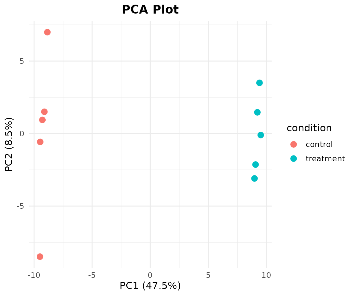
Add shape mapping and sample labels:
bb_pca(cpm, metadata, color_by = "condition", shape_by = "batch", label = TRUE)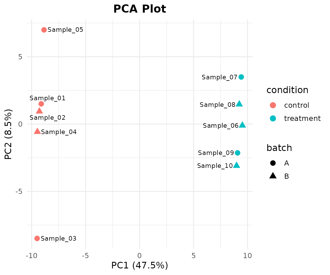
Step 5: Differential Expression
Option A: With DESeq2 (requires Bioconductor)
de_results <- bb_deseq2(counts, metadata)
#> estimating size factors
#> estimating dispersions
#> gene-wise dispersion estimates
#> mean-dispersion relationship
#> -- note: fitType='parametric', but the dispersion trend was not well captured by the
#>    function: y = a/x + b, and a local regression fit was automatically substituted.
#>    specify fitType='local' or 'mean' to avoid this message next time.
#> final dispersion estimates
#> fitting model and testing
head(de_results[order(de_results$padj), ])
#>     gene   log2fc pvalue padj  basemean
#> 1   TP53 1.620871      0    0 1050.8776
#> 3   EGFR 1.619625      0    0 1001.6421
#> 5 PIK3CA 1.582527      0    0  983.2855
#> 7    APC 1.617024      0    0 1100.7746
#> 8 CDKN2A 1.584825      0    0 1011.5725
#> 9    RB1 1.548702      0    0 1055.2935
Option B: Use Pre-computed DE Results (no Bioconductor!)
bambamR bundles a realistic pre-computed DE result set so you can explore all downstream plots without installing Bioconductor:
de_results <- bb_example_de()
head(de_results[order(de_results$padj), ])
#>     gene   log2fc       pvalue       padj   basemean
#> 1   TP53 2.339649 0.0007574367 0.02349398  997.58686
#> 2   KRAS 2.722469 0.0003361832 0.02349398   90.62812
#> 3   EGFR 2.444921 0.0008361128 0.02349398   47.01289
#> 4   BRAF 1.623780 0.0005590749 0.02349398  179.27216
#> 5 PIK3CA 1.271091 0.0004387668 0.02349398   12.32381
#> 6   PTEN 2.006420 0.0006551589 0.02349398 9793.59126
cat("Total genes:", nrow(de_results), "\n")
#> Total genes: 500
cat("Significant (padj < 0.05):", sum(de_results$padj < 0.05, na.rm = TRUE), "\n")
#> Significant (padj < 0.05): 20
cat("Up-regulated (log2FC > 1):",
    sum(de_results$padj < 0.05 & de_results$log2fc > 1, na.rm = TRUE), "\n")
#> Up-regulated (log2FC > 1): 10
cat("Down-regulated (log2FC < -1):",
    sum(de_results$padj < 0.05 & de_results$log2fc < -1, na.rm = TRUE), "\n")
#> Down-regulated (log2FC < -1): 10
Step 6: Volcano Plot
bb_volcano(de_results, fc_cutoff = 1, p_cutoff = 0.05, n_label = 8)
#> Warning: Removed 492 rows containing missing values or values outside the scale range
#> (`geom_text_repel()`).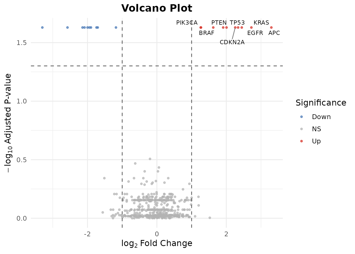
Customize the cutoffs and label specific genes:
bb_volcano(de_results,
           fc_cutoff = 0.5,
           p_cutoff = 0.01,
           label_genes = c("TP53", "KRAS", "EGFR", "PTEN"),
           colors = c(up = "#E41A1C", down = "#377EB8", ns = "grey80"))
#> Warning: Removed 496 rows containing missing values or values outside the scale range
#> (`geom_text_repel()`).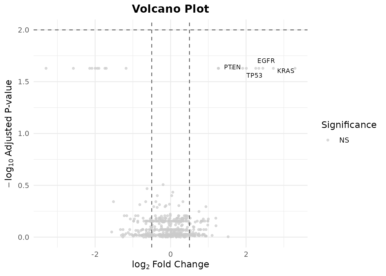
Step 7: MA Plot
The MA plot shows log2 fold-change vs. mean expression, highlighting genes that change at different expression levels:
bb_ma_plot(de_results, p_cutoff = 0.05)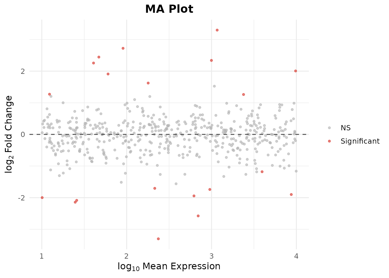
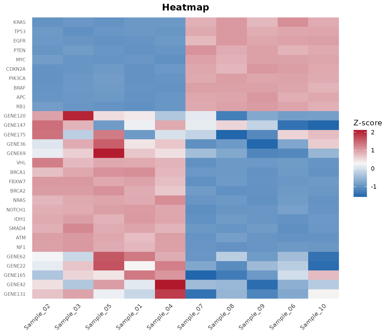
Step 8: Heatmap of Top DE Genes
Pass DE results to bb_heatmap() to show the top
differentially expressed genes instead of the most variable:
bb_heatmap(cpm, de_result = de_results, n_genes = 25)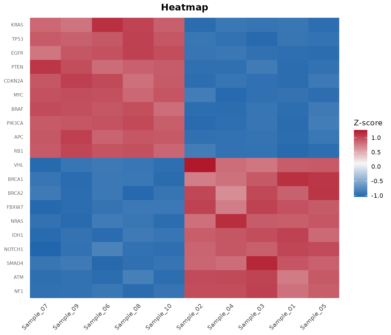
Step 9: Oncoplot
The oncoplot is bambamR’s signature visualization – a waterfall-style mutation landscape across samples. Load the bundled mutation data:
mut <- bb_example_mutations()
head(mut$mutations)
#>     sample   gene     mutation_type
#> 1 TCGA-021   NRAS      In_Frame_Ins
#> 2 TCGA-037 PIK3CA Missense_Mutation
#> 3 TCGA-037   BRAF       Splice_Site
#> 4 TCGA-031 PIK3CA   Frame_Shift_Ins
#> 5 TCGA-042    RB1 Missense_Mutation
#> 6 TCGA-008   NRAS Missense_Mutation
head(mut$clinical)
#>          Stage Gender Smoking
#> TCGA-021   III   Male  Former
#> TCGA-037     I   Male   Never
#> TCGA-031    II Female   Never
#> TCGA-042   III Female Current
#> TCGA-008    IV Female  Former
#> TCGA-029   III Female  Former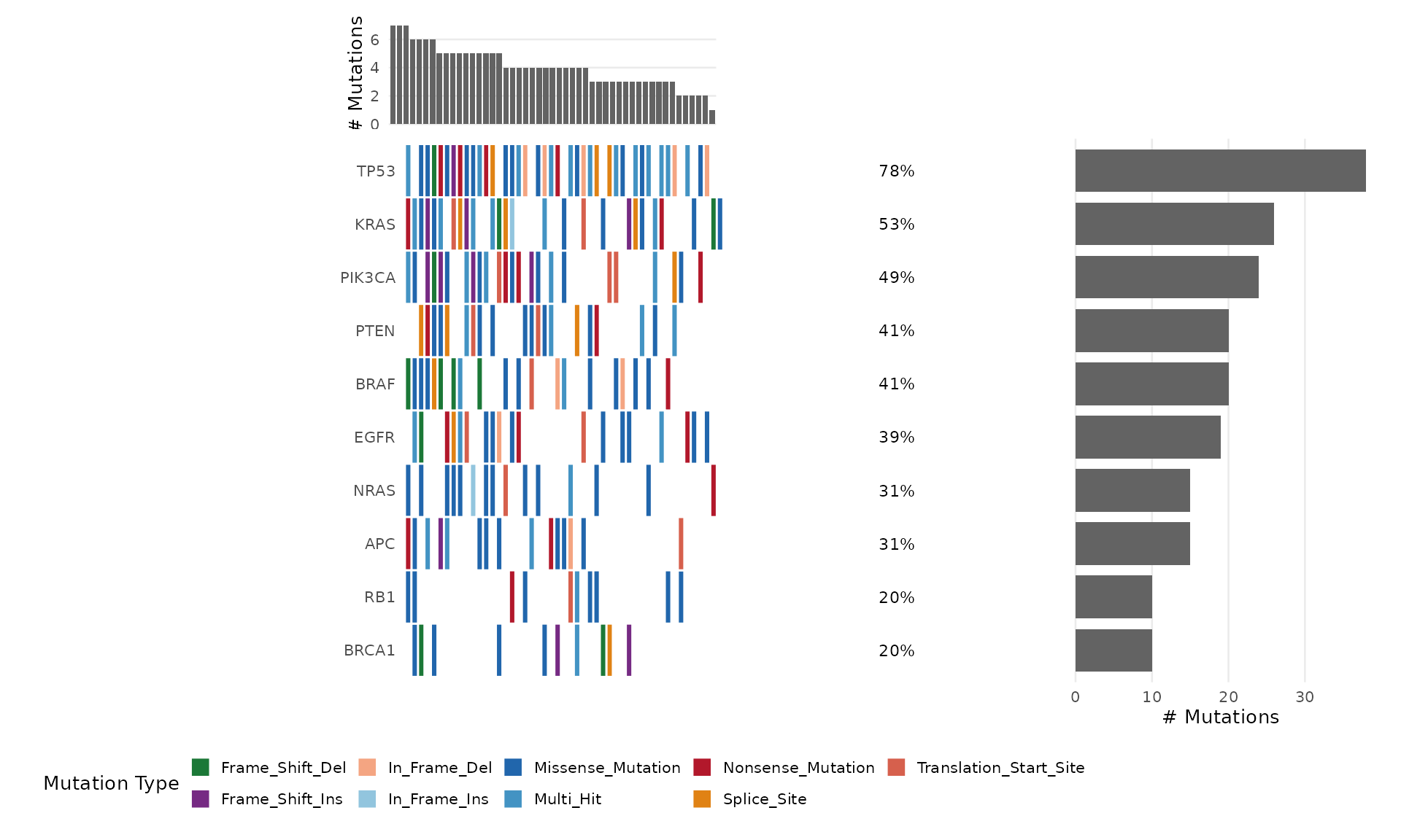
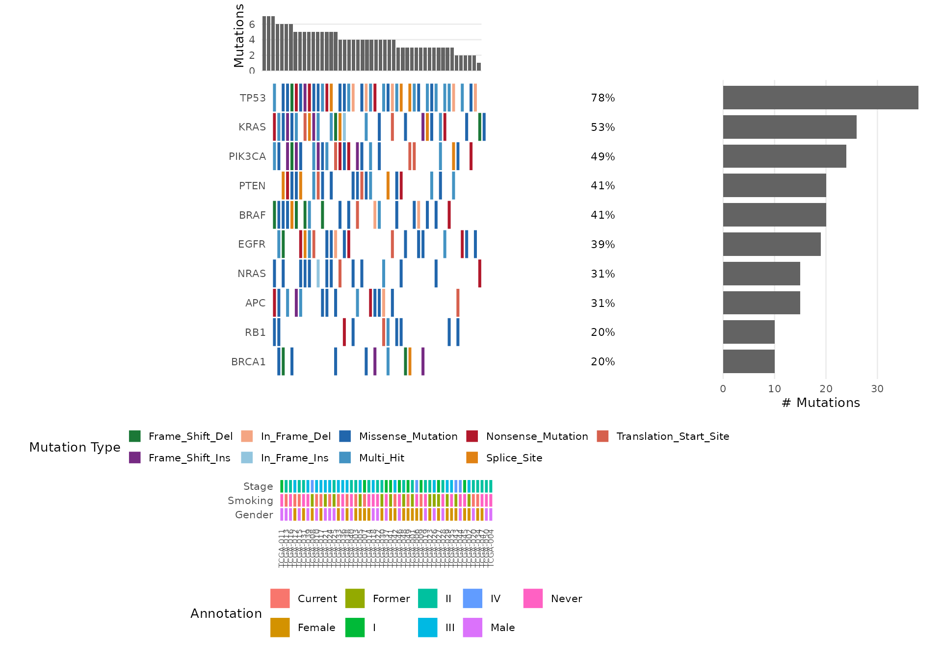
Select Specific Genes
bb_oncoplot(mut$mutations,
            genes = c("TP53", "KRAS", "PIK3CA", "BRAF", "EGFR"))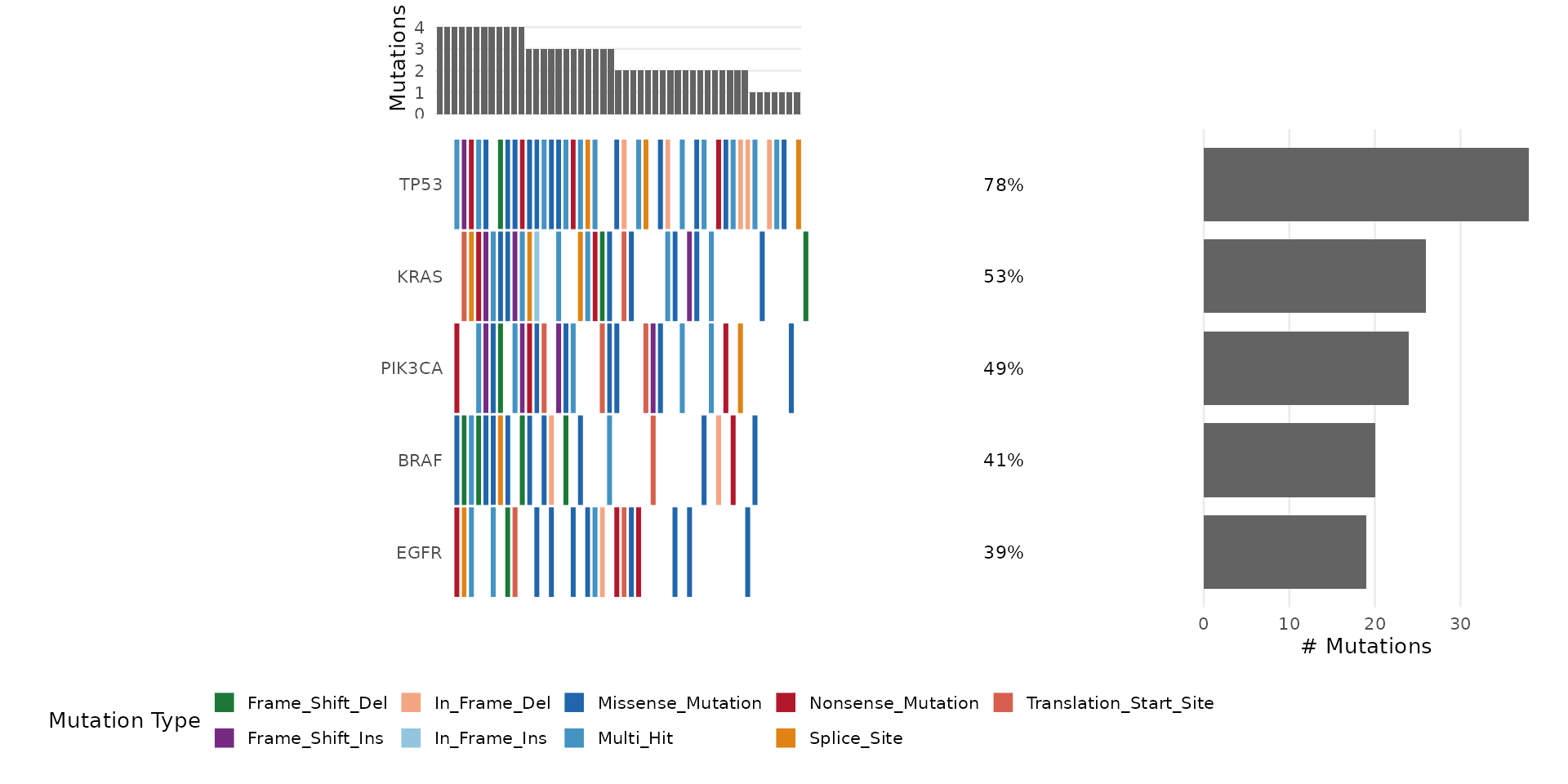
See vignette("bambamR-oncoplot") for more customization
options.
Step 10: Read FASTQ Files
bambamR includes a small example FASTQ file (100 reads):
fq_path <- system.file("extdata", "example_reads.fastq", package = "bambamR")
reads <- bb_read_fastq(fq_path, n = 5)
reads
#>                    id
#> 1 read_0001 length=75
#> 2 read_0002 length=75
#> 3 read_0003 length=75
#> 4 read_0004 length=75
#> 5 read_0005 length=75
#>                                                                      sequence
#> 1 CCCTAGATGAGTGGATTCACCTATCGGCGGTATATGTTTCGAAATCTGAGACGCAAAGACCTGTATAAAATTCCC
#> 2 GCGAAGGGATAATAGTCCCTACGAATCTGAAAATGACTAACATGCGTTAGCAACGGTACTGATGGGTATAGGTCA
#> 3 AGGAGTGTTTAACCGGTGACAGCGCCTAATTCTGGAGGGTGGTACCACACACCAACATTACAGATCCGACGACAT
#> 4 ACTAGTCAGGAATCATGTGTGTGATTCCATAGACACATGGCGCGGAAGCCGGCCATATCCCCGTAACGAGCCGCC
#> 5 CGTTCGGCAGATCTACCGGTGTGACTTGACCGGCATTGCTCACCAGAAAGAGTGTAGTTGCCTGAGCCTGTAATG
#>                                                                       quality
#> 1 >FEGGCIHGFDIEEIHGIIGEFFDCEFGCBEAIIIEGF=IDEEHEFBGAGCIBICIBHCDIHHEGHGA?GEGCCG
#> 2 HGIBCGDHGAIEGADGHFFAIIEFIIHFBIGHBIFFBDGFDFEIHIAFD=HHC=HHIGGFICH=HDIHHHCEIIB
#> 3 GHEEHHBABGDHDIFGFFEEGGHIGFEDHEIEDFFIHDGHE>AICHHE>GBHECFCH?EHEIGDEEICCEGIIHH
#> 4 EE?IGFFIEGFIEIGIHEIIHDHGHEEHFGIHHGFGFCFIHHAIEFHFBHHHAHGHI>EIBFHDIHFFIHHBHFE
#> 5 EIGCIIEGHGIDHEICGEDHCGEGHEEHIHDHGIHAEEFGIEIB=IFDBIBEGFIGIIIHAEG?DIGIBIFHFHG
all_reads <- bb_read_fastq(fq_path)
cat("Total reads:", nrow(all_reads), "\n")
#> Total reads: 100
cat("Read length:", nchar(all_reads$sequence[1]), "bp\n")
#> Read length: 75 bp
Step 11: Quality Control
Run QC on the example FASTQ file:
qc <- bb_qc(fastq_path = fq_path)
qc
#> bambamR QC Summary
#> ==================
#> Files analyzed: 1
#>   example_reads.fastq: 100 reads
bb_qc_summary(qc)
#>                  file total_reads median_gc mapping_rate
#> 1 example_reads.fastq         100 0.4933333           NA
Visualize QC metrics:
bb_plot_qc(qc)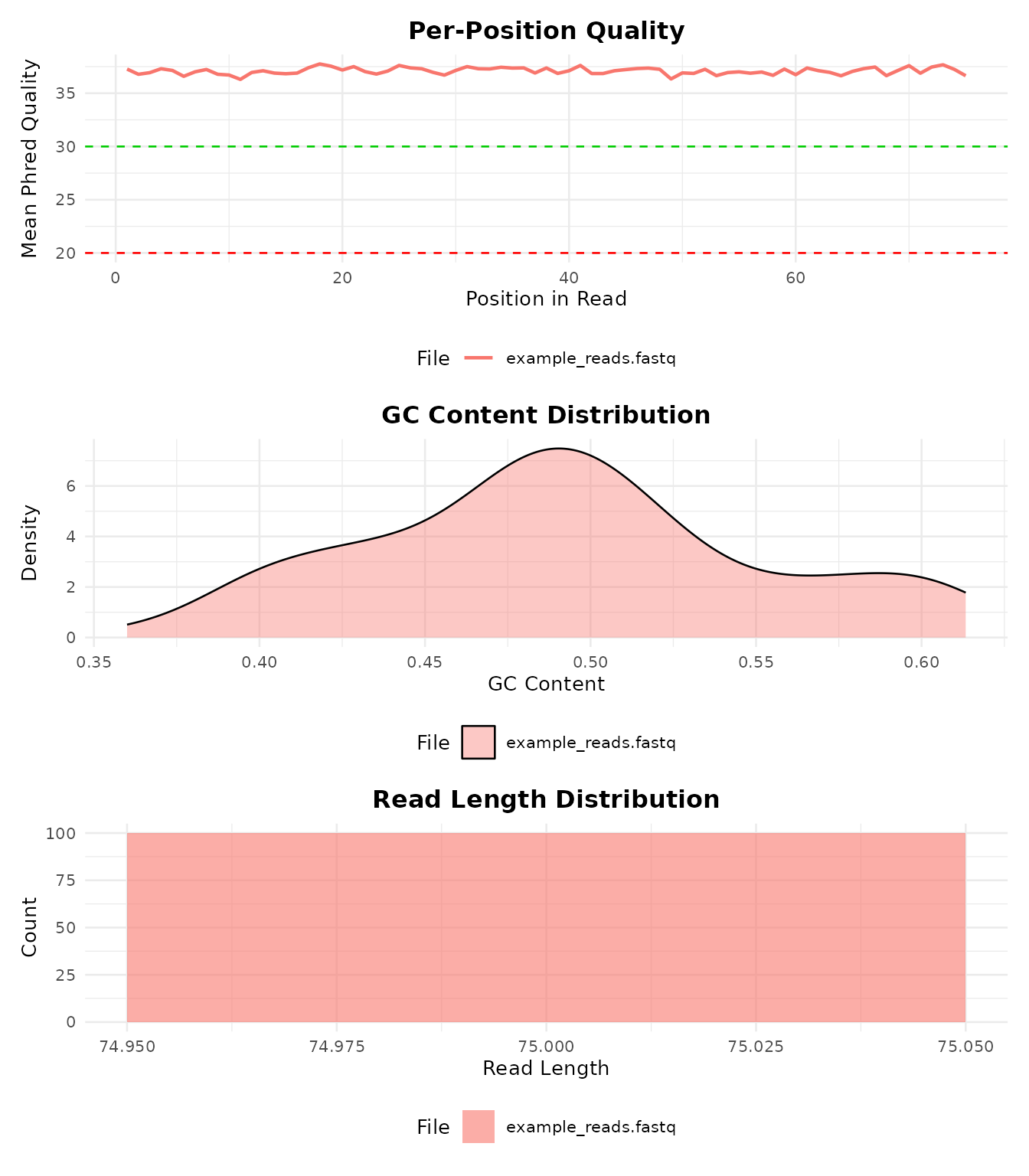
Step 12: Export Results
Save your results in various formats:
# Save DE results as CSV / TSV
bb_export_csv(de_results, "de_results.csv")
bb_export_tsv(de_results, "de_results.tsv")

# Save the full analysis as RDS (preserves R objects)
bb_export_rds(de_results, "de_results.rds")
Full Pipeline (FASTQ to Plots in One Call)
When you have real data (FASTQ files, a genome index, and a GTF annotation), run the entire pipeline with a single function:
result <- bb_pipeline(
  fastq_dir    = "raw_reads/",
  genome_index = "STAR_index/",
  annotation   = "genes.gtf",
  sample_info  = metadata,
  aligner      = "STAR",
  de_method    = "DESeq2",
  threads      = 8
)

# Access results
result$counts          # count matrix
result$de_results      # DE data.frame
result$plots$pca       # ggplot object
result$plots$volcano   # ggplot object
result$plots$heatmap   # ggplot object
You can enter the pipeline at any stage:
# From BAM files (skip alignment)
result <- bb_pipeline(
  bam_dir    = "aligned/",
  annotation = "genes.gtf",
  sample_info = metadata
)

# From a count matrix (skip alignment + counting)
result <- bb_pipeline(
  count_matrix = my_counts,
  sample_info  = metadata,
  de_method    = "edgeR"
)
Interactive Shiny App
For a point-and-click interface, launch the Shiny app:
The app lets you upload data, configure parameters, run the analysis, and interactively explore volcano plots, heatmaps, PCA, and onco plots. You can export results as CSV, RDS, or PDF directly from the browser.
What’s Next?
-
vignette("bambamR-oncoplot")– detailed oncoplot customization -
?bb_pipeline– full pipeline documentation -
?bb_deseq2,?bb_edger,?bb_limma_voom– DE method details