5-Minute Tutorial: RNA-Seq Analysis with bambamR

This tutorial walks through a complete RNA-seq analysis in under 5 minutes using only bambamR’s built-in example data. No Bioconductor packages are required.

Load the Package

library(bambamR)
#> bambamR: Full mode (all Bioconductor packages available)

1. Load Data and Normalize

# Bundled example: 200 genes x 10 samples (5 control, 5 treatment)
ex <- bb_example_counts()
cpm <- bb_normalize(ex$counts, method = "cpm")
cat(nrow(cpm), "genes,", ncol(cpm), "samples\n")
#> 200 genes, 10 samples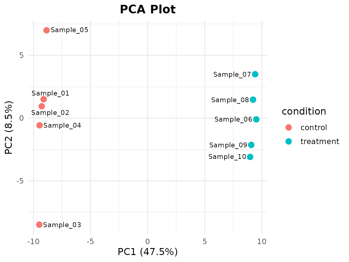

2. PCA: Do the Groups Separate?

bb_pca(cpm, ex$metadata, color_by = "condition", label = TRUE)

3. Volcano Plot: What Changed?

Use the pre-computed DE results (no Bioconductor needed):

de <- bb_example_de()
bb_volcano(de, fc_cutoff = 1, p_cutoff = 0.05, n_label = 6)
#> Warning: Removed 494 rows containing missing values or values outside the scale range
#> (`geom_text_repel()`).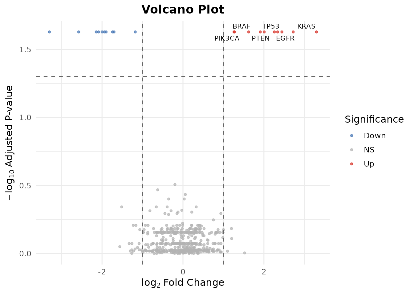

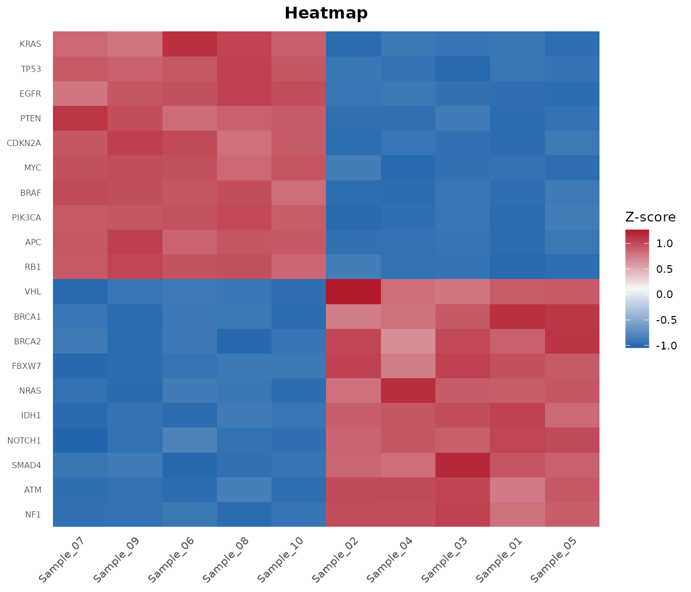
4. MA Plot: Effect vs. Expression

bb_ma_plot(de)

5. Heatmap: Top DE Genes

bb_heatmap(cpm, de_result = de, n_genes = 20)

6. Oncoplot: Mutation Landscape

mut <- bb_example_mutations()
bb_oncoplot(mut$mutations, n_genes = 10, annotation_df = mut$clinical)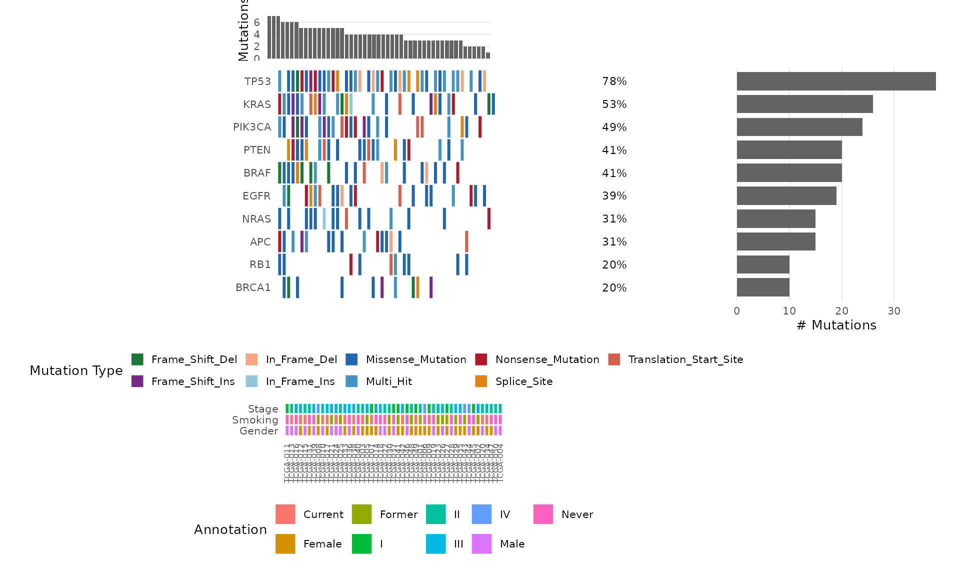

7. Export

bb_export_csv(de, "my_results.csv")

Done!

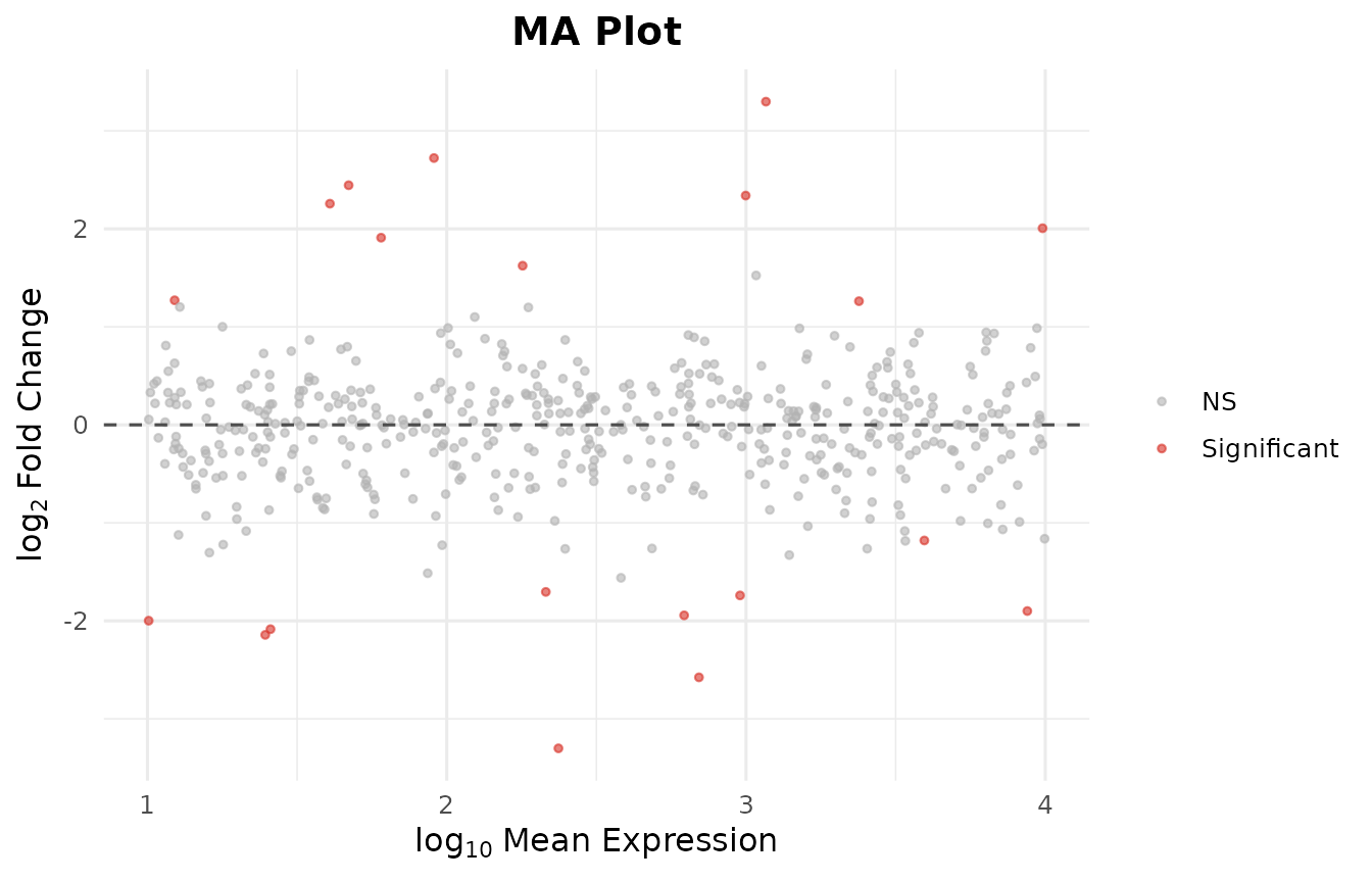
In 7 steps you went from a count matrix to publication-ready PCA, volcano, MA, heatmap, and onco plots – all without Bioconductor.

What’s next?

• With Bioconductor: bb_deseq2(), bb_edger(), bb_limma_voom() for real DE analysis
• From raw data: bb_pipeline() handles FASTQ -> alignment -> counts -> DE -> plots
• Interactive: bb_run_app() launches a Shiny dashboard
• Customization: every plot returns a ggplot2 object, so add + theme(), + labs(), + scale_*() as needed
• See vignette("bambamR-quickstart") for the full walkthrough and vignette("bambamR-oncoplot") for oncoplot customization