bambamR: End-to-End RNA-Seq Processing from FASTQ to Publication-Ready Plots

Introduction

bambamR is an R package for end-to-end RNA-seq analysis. It covers the full pipeline from raw FASTQ/BAM files through quality control, alignment, read counting, normalization, differential expression analysis, and publication-ready visualizations including onco plots, volcano plots, heatmaps, PCA, and MA plots.

Key Design Principles

Graceful degradation: All Bioconductor dependencies are optional. The package operates in minimal mode (CRAN-only) or full mode (with Bioconductor). It never breaks if Bioconductor is missing.
Consistent interface: All exported functions use the bb_ prefix. All plot functions return ggplot2 objects for easy customization.
Bundled example data: Every feature can be explored without downloading external files or installing Bioconductor.

Minimal vs. Full Mode

Feature	Minimal (CRAN)	Full (+ Bioconductor)
CPM / TPM normalization	Yes	Yes
TMM / RLE normalization	–	Yes
DESeq2 / edgeR / limma	–	Yes
PCA, volcano, heatmap, MA	Yes	Yes
Onco plots	Yes	Yes
FASTQ / BAM import	Base-R	ShortRead / Rsamtools
Alignment wrappers	Yes	Yes
Read counting	featureCounts CLI	GenomicAlignments
Shiny interactive app	Yes	Yes

Installation

Install from CRAN (when available):

install.packages("bambamR")

Install the development version from GitHub:

pak::pak("r-heller/bambamR")

Optionally install Bioconductor packages for full-mode features:

BiocManager::install(c(
  "DESeq2", "edgeR", "limma",
  "ShortRead", "Rsamtools",
  "GenomicAlignments", "GenomicRanges"
))

library(bambamR)

Bundled Example Data

bambamR ships with ready-to-use datasets accessible via convenience functions:

Function	Contents
`bb_example_counts()`	200 genes x 10 samples + metadata
`bb_example_mutations()`	300 mutations, 50 samples, 20 genes + clinical data
`bb_example_de()`	500-gene pre-computed DE results

# RNA-seq count matrix (200 genes x 10 samples)
ex <- bb_example_counts()
counts   <- ex$counts
metadata <- ex$metadata

dim(counts)
#> [1] 200  10
counts[1:5, 1:5]
#>        Sample_01 Sample_02 Sample_03 Sample_04 Sample_05
#> TP53         525       533       485       515       519
#> KRAS         502       471       498       510       475
#> EGFR         479       504       488       514       473
#> BRAF         454       456       481       453       497
#> PIK3CA       470       469       506       483       532

metadata
#>           condition batch sex age
#> Sample_01   control     A   M  45
#> Sample_02   control     B   F  52
#> Sample_03   control     A   M  38
#> Sample_04   control     B   F  61
#> Sample_05   control     A   M  55
#> Sample_06 treatment     B   F  47
#> Sample_07 treatment     A   M  59
#> Sample_08 treatment     B   F  42
#> Sample_09 treatment     A   M  50
#> Sample_10 treatment     B   F  44

Normalization

CPM (Counts Per Million)

CPM normalization works without any optional dependencies:

cpm <- bb_normalize(counts, method = "cpm")

TPM (Transcripts Per Million)

TPM requires gene lengths:

gene_lengths <- readRDS(
  system.file("extdata", "example_gene_lengths.rds", package = "bambamR")
)
tpm <- bb_normalize(counts, method = "tpm",
                    gene_lengths = gene_lengths$length)

TMM and RLE (Bioconductor)

With Bioconductor installed:

tmm <- bb_normalize(counts, method = "tmm")  # requires edgeR
rle <- bb_normalize(counts, method = "rle")  # requires DESeq2

Visualization

All plot functions return ggplot2 objects that can be further customized with + theme(), + labs(), etc.

PCA Plot

bb_pca(cpm, metadata, color_by = "condition")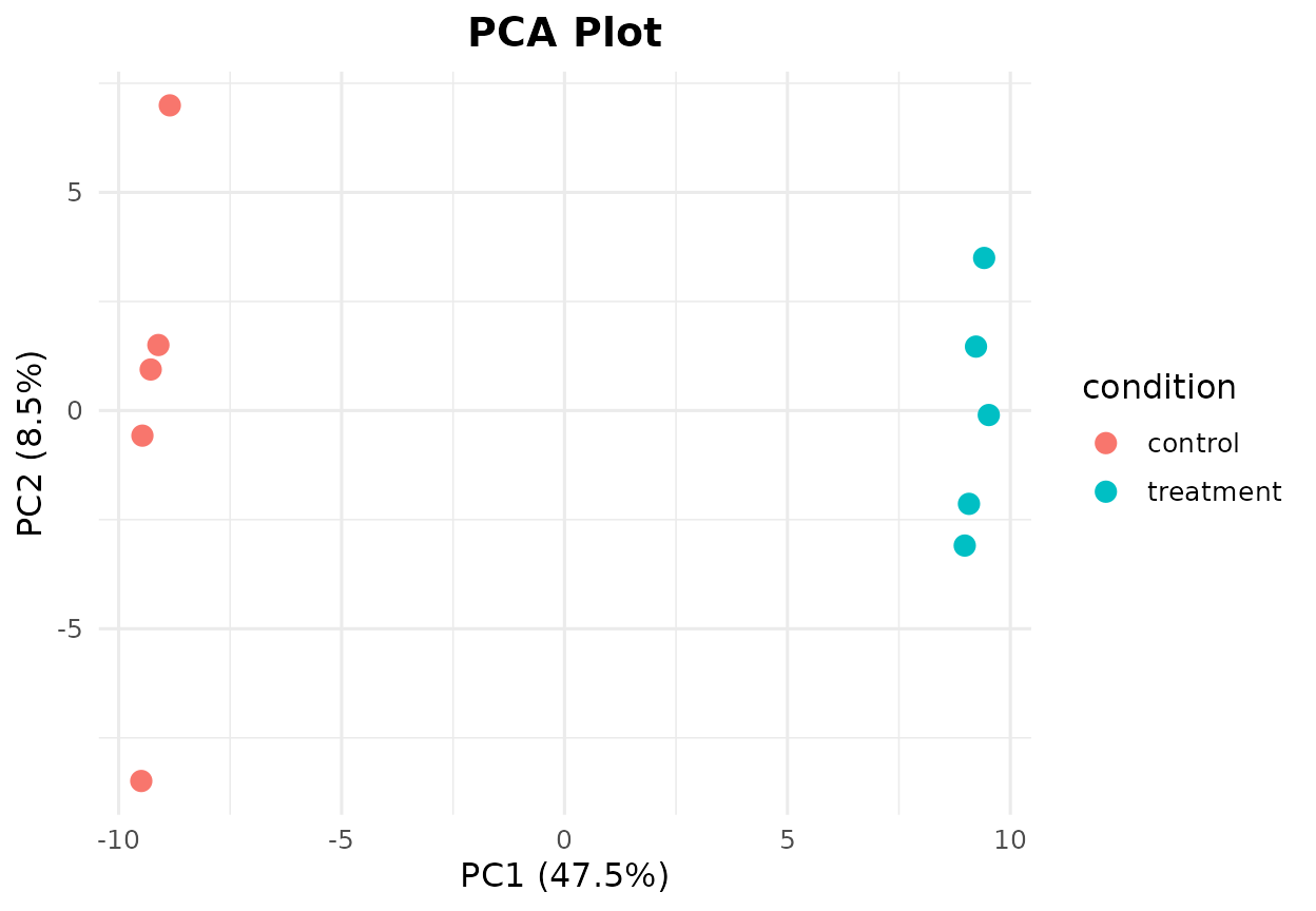

PCA plot colored by experimental condition.

bb_pca(cpm, metadata, color_by = "condition",
       shape_by = "batch", label = TRUE, point_size = 4)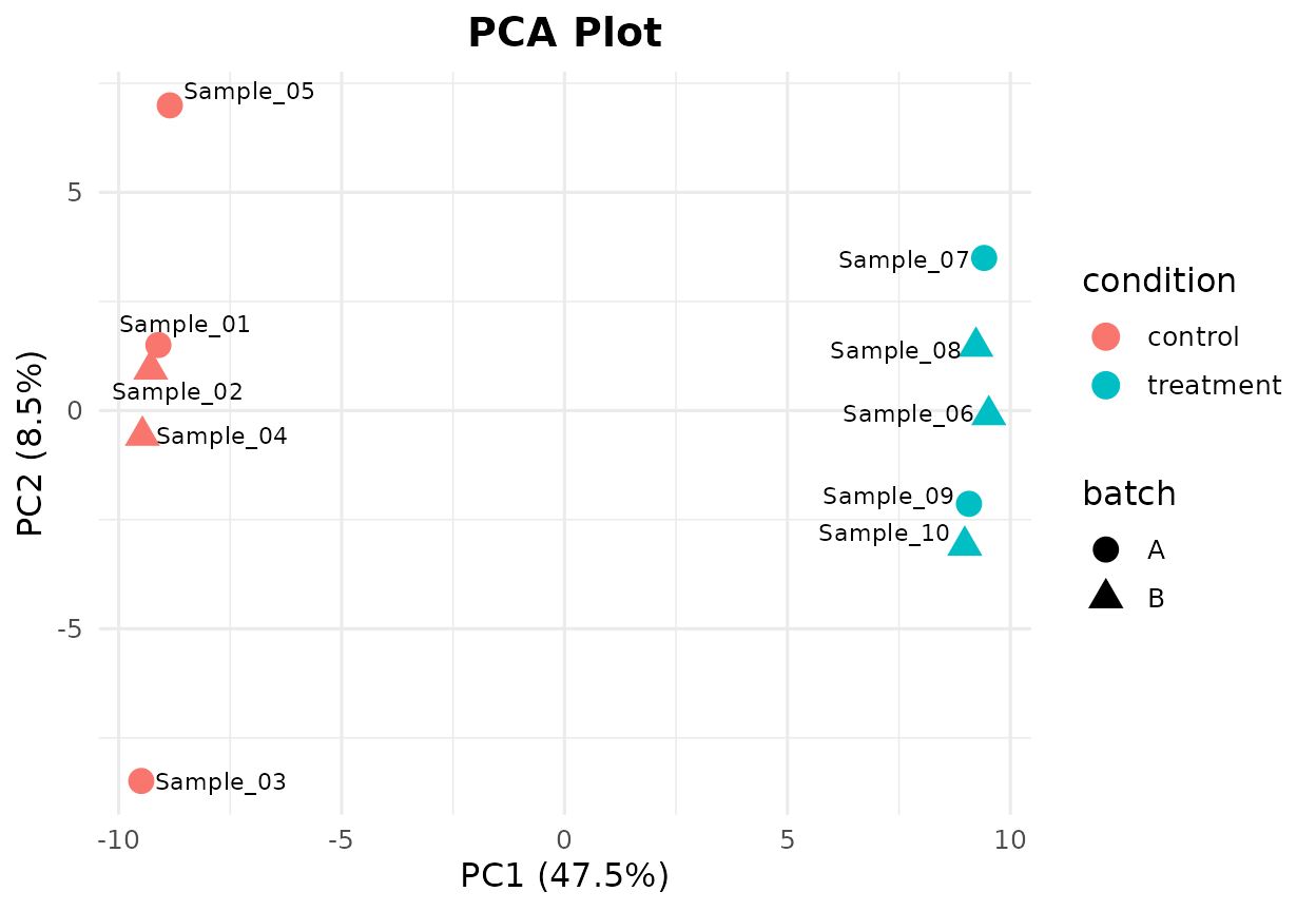

PCA plot with shape mapping for batch effect.

Heatmap

bb_heatmap(cpm, n_genes = 30)

Heatmap of the 30 most variable genes.

Volcano Plot

Using the pre-computed DE results (no Bioconductor required):

de_results <- bb_example_de()
sig <- sum(de_results$padj < 0.05, na.rm = TRUE)
cat("Significant genes (FDR < 0.05):", sig, "\n")
#> Significant genes (FDR < 0.05): 20

bb_volcano(de_results, fc_cutoff = 1, p_cutoff = 0.05, n_label = 8)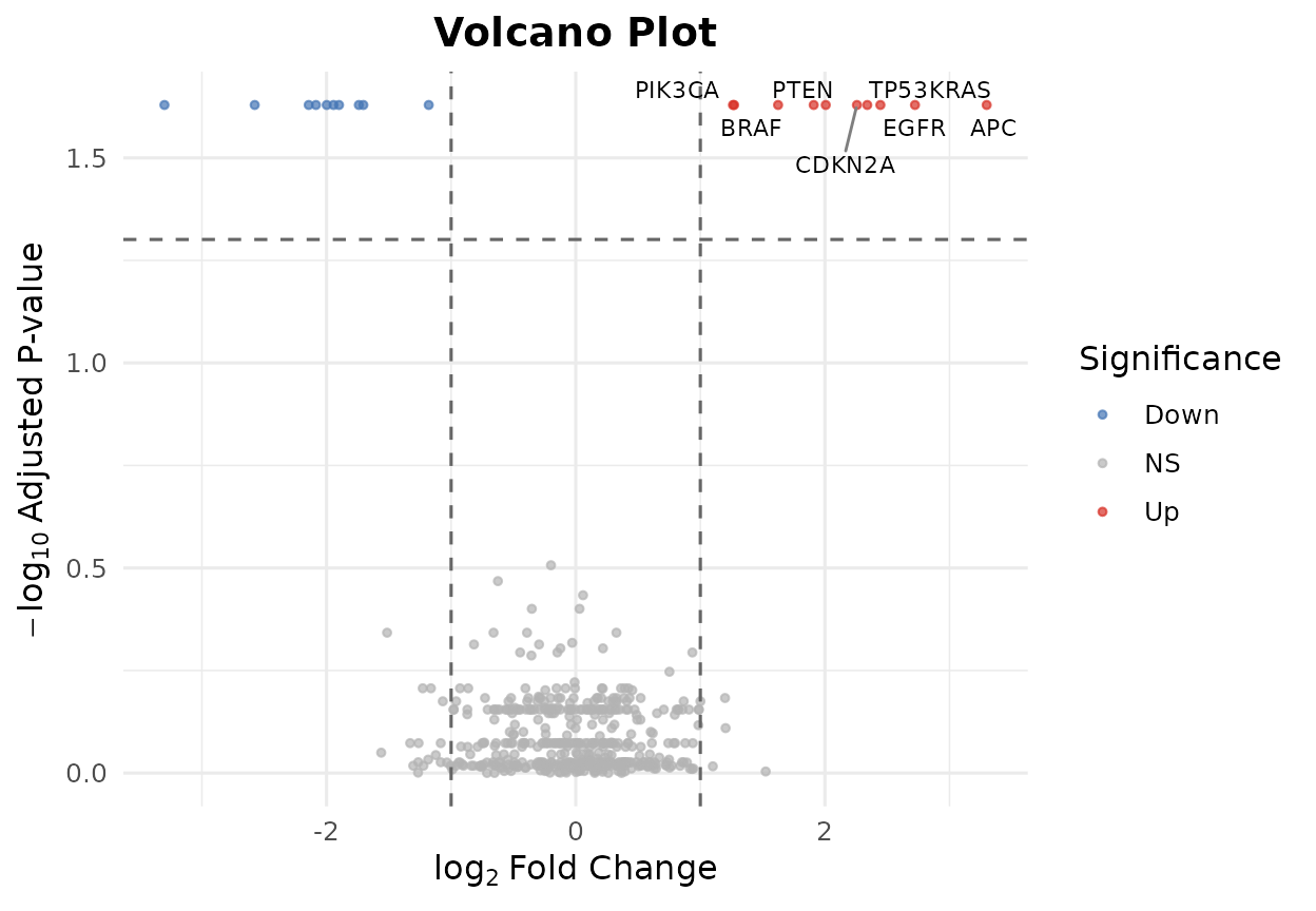

Volcano plot highlighting differentially expressed genes.

bb_volcano(de_results,
           fc_cutoff = 0.5,
           p_cutoff = 0.01,
           label_genes = c("TP53", "KRAS", "EGFR", "PTEN"),
           colors = c(up = "#E41A1C", down = "#377EB8", ns = "grey80"))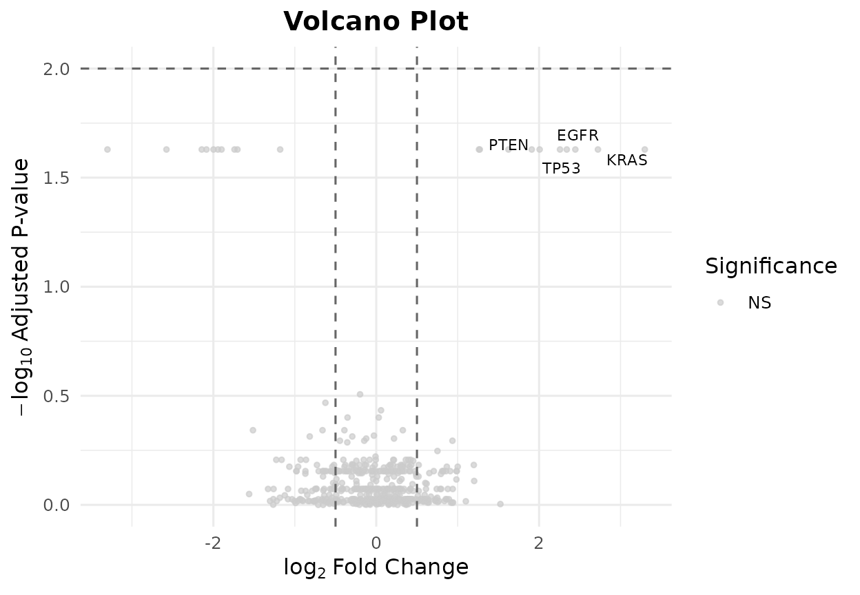

Volcano plot with custom gene labels and colors.

MA Plot

bb_ma_plot(de_results, p_cutoff = 0.05)

MA plot showing fold-change vs.~mean expression.

Heatmap of Top DE Genes

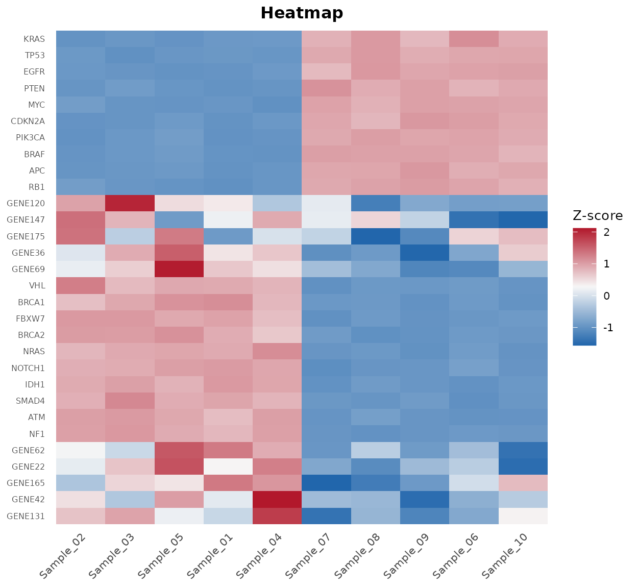
bb_heatmap(cpm, de_result = de_results, n_genes = 25)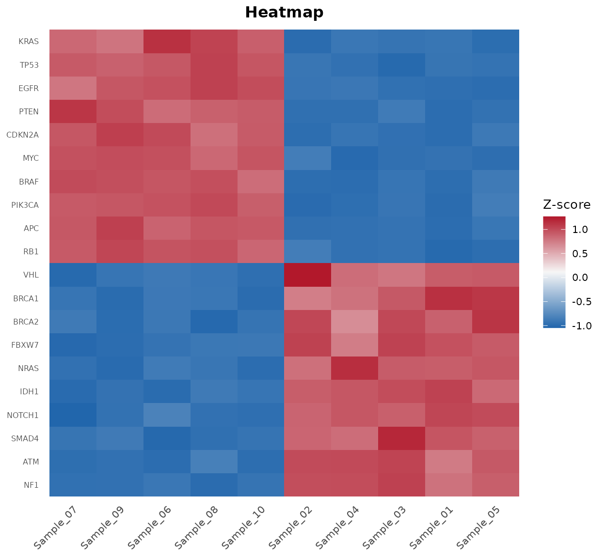

Heatmap of the top 25 differentially expressed genes.

Oncoplot

The bb_oncoplot() function creates publication-ready waterfall-style mutation landscape plots.

Data Format

bambamR accepts a data.frame with columns sample, gene, and mutation_type, or MAF-format data with Hugo_Symbol, Tumor_Sample_Barcode, and Variant_Classification.

mut <- bb_example_mutations()
head(mut$mutations)
#>     sample   gene     mutation_type
#> 1 TCGA-021   NRAS      In_Frame_Ins
#> 2 TCGA-037 PIK3CA Missense_Mutation
#> 3 TCGA-037   BRAF       Splice_Site
#> 4 TCGA-031 PIK3CA   Frame_Shift_Ins
#> 5 TCGA-042    RB1 Missense_Mutation
#> 6 TCGA-008   NRAS Missense_Mutation

Basic Oncoplot

bb_oncoplot(mut$mutations, n_genes = 10, show_barplot = FALSE)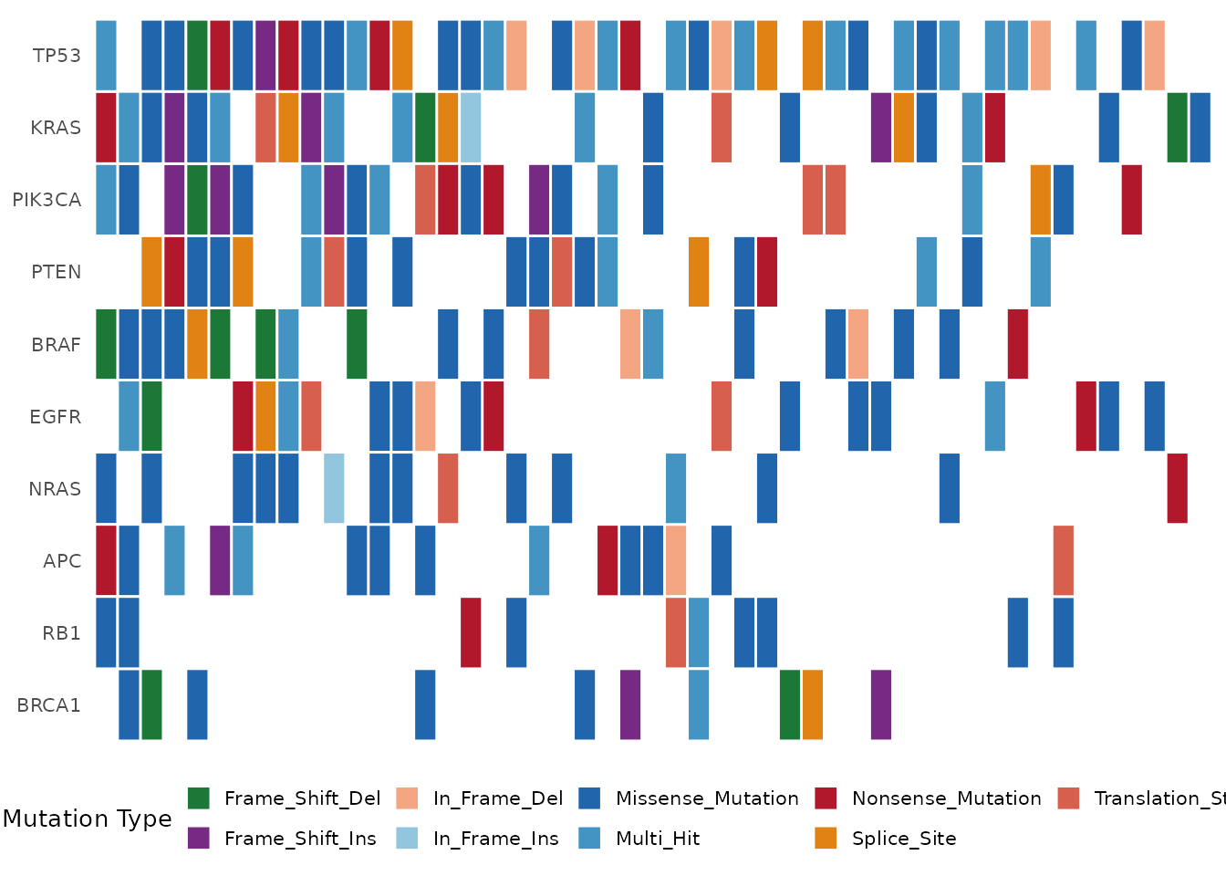

Oncoplot showing the top 10 mutated genes.

Oncoplot with Clinical Annotations

bb_oncoplot(mut$mutations, n_genes = 8,
            annotation_df = mut$clinical, show_barplot = FALSE)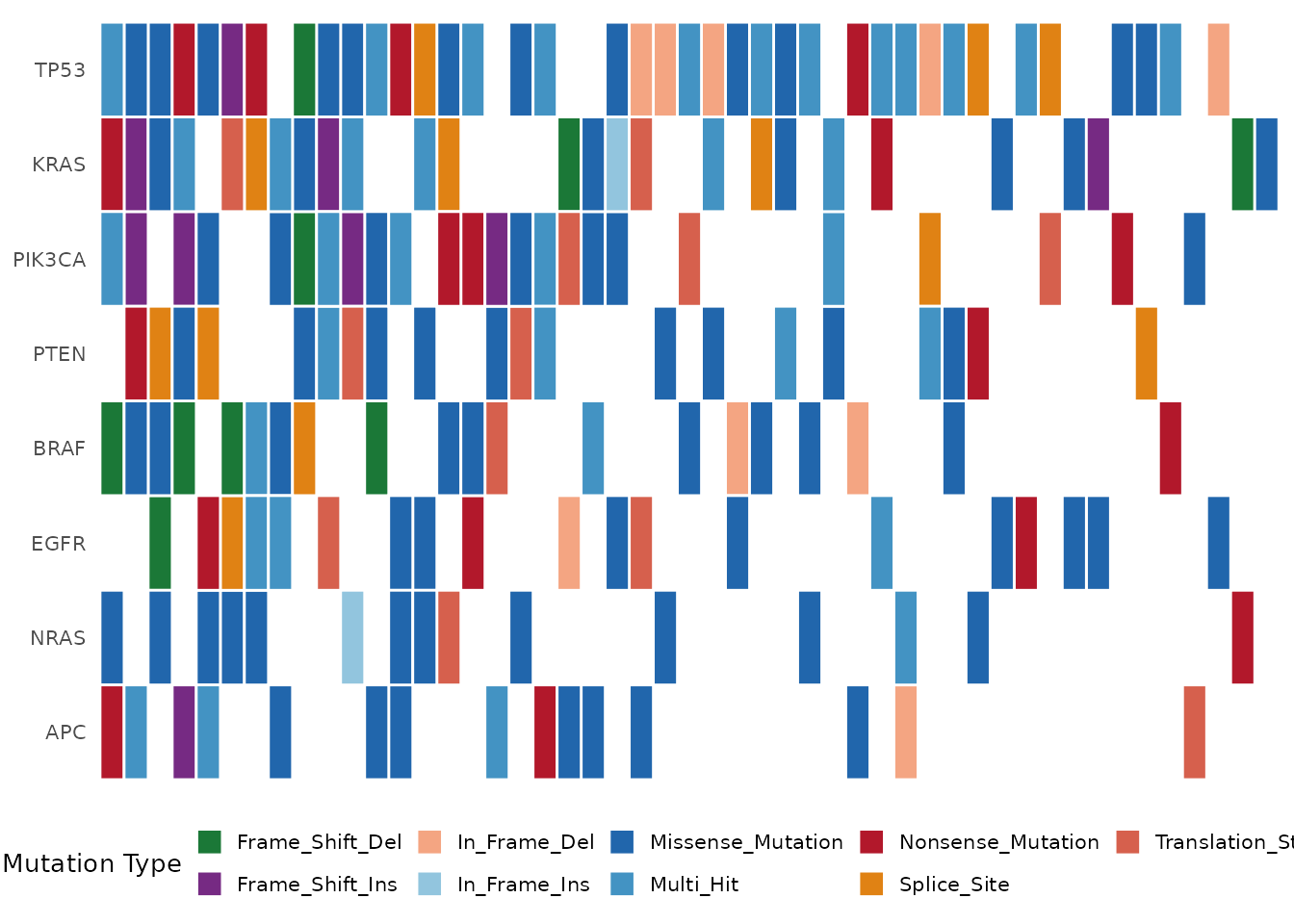

Oncoplot with clinical annotation tracks (Stage, Gender, Smoking).

Selecting Specific Genes

bb_oncoplot(mut$mutations, show_barplot = FALSE,
            genes = c("TP53", "KRAS", "PIK3CA", "BRAF", "EGFR"))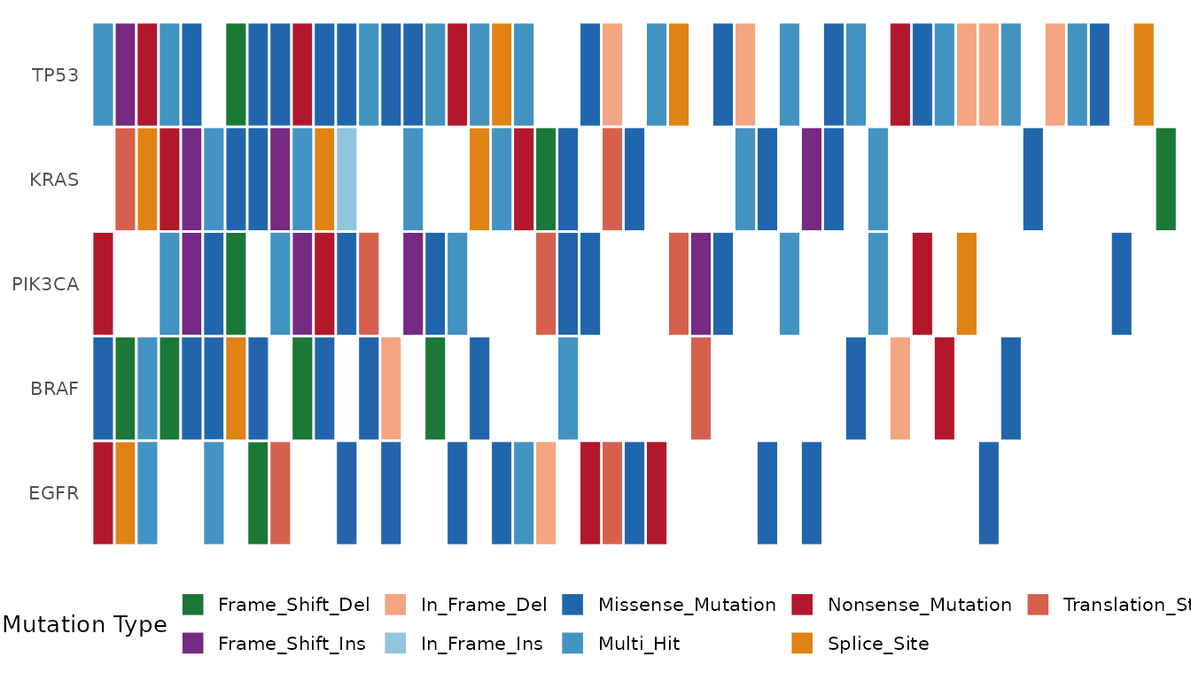

Oncoplot showing five selected genes.

Custom Colors

my_colors <- c(
  "Missense_Mutation" = "#3182BD",
  "Nonsense_Mutation" = "#E6550D",
  "Frame_Shift_Del"   = "#31A354",
  "Frame_Shift_Ins"   = "#756BB1",
  "Splice_Site"       = "#DE2D26",
  "In_Frame_Del"      = "#636363",
  "In_Frame_Ins"      = "#FDAE6B",
  "Translation_Start_Site" = "#BCBDDC",
  "Multi_Hit"         = "#FDD0A2",
  "Other"             = "#BDBDBD"
)
bb_oncoplot(mut$mutations, n_genes = 8,
            mutation_colors = my_colors, show_barplot = FALSE)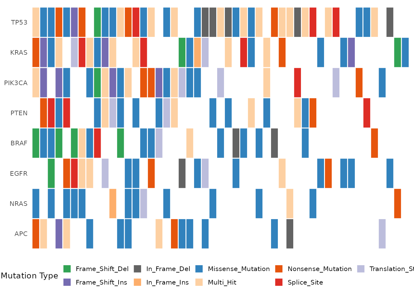

Oncoplot with a custom color palette.

FASTQ Import

bambamR includes a small example FASTQ file (100 reads, 75 bp):

fq_path <- system.file("extdata", "example_reads.fastq",
                        package = "bambamR")
reads <- bb_read_fastq(fq_path, n = 5)
reads
#>                    id
#> 1 read_0001 length=75
#> 2 read_0002 length=75
#> 3 read_0003 length=75
#> 4 read_0004 length=75
#> 5 read_0005 length=75
#>                                                                      sequence
#> 1 CCCTAGATGAGTGGATTCACCTATCGGCGGTATATGTTTCGAAATCTGAGACGCAAAGACCTGTATAAAATTCCC
#> 2 GCGAAGGGATAATAGTCCCTACGAATCTGAAAATGACTAACATGCGTTAGCAACGGTACTGATGGGTATAGGTCA
#> 3 AGGAGTGTTTAACCGGTGACAGCGCCTAATTCTGGAGGGTGGTACCACACACCAACATTACAGATCCGACGACAT
#> 4 ACTAGTCAGGAATCATGTGTGTGATTCCATAGACACATGGCGCGGAAGCCGGCCATATCCCCGTAACGAGCCGCC
#> 5 CGTTCGGCAGATCTACCGGTGTGACTTGACCGGCATTGCTCACCAGAAAGAGTGTAGTTGCCTGAGCCTGTAATG
#>                                                                       quality
#> 1 >FEGGCIHGFDIEEIHGIIGEFFDCEFGCBEAIIIEGF=IDEEHEFBGAGCIBICIBHCDIHHEGHGA?GEGCCG
#> 2 HGIBCGDHGAIEGADGHFFAIIEFIIHFBIGHBIFFBDGFDFEIHIAFD=HHC=HHIGGFICH=HDIHHHCEIIB
#> 3 GHEEHHBABGDHDIFGFFEEGGHIGFEDHEIEDFFIHDGHE>AICHHE>GBHECFCH?EHEIGDEEICCEGIIHH
#> 4 EE?IGFFIEGFIEIGIHEIIHDHGHEEHFGIHHGFGFCFIHHAIEFHFBHHHAHGHI>EIBFHDIHFFIHHBHFE
#> 5 EIGCIIEGHGIDHEICGEDHCGEGHEEHIHDHGIHAEEFGIEIB=IFDBIBEGFIGIIIHAEG?DIGIBIFHFHG

When ShortRead is available, bb_read_fastq() uses it automatically. Otherwise, a base-R parser handles plain and gzipped FASTQ files.

Quality Control

qc <- bb_qc(fastq_path = fq_path)
qc
#> bambamR QC Summary
#> ==================
#> Files analyzed: 1 
#>   example_reads.fastq: 100 reads

bb_qc_summary(qc)
#>                  file total_reads median_gc mapping_rate
#> 1 example_reads.fastq         100 0.4933333           NA

bb_plot_qc(qc)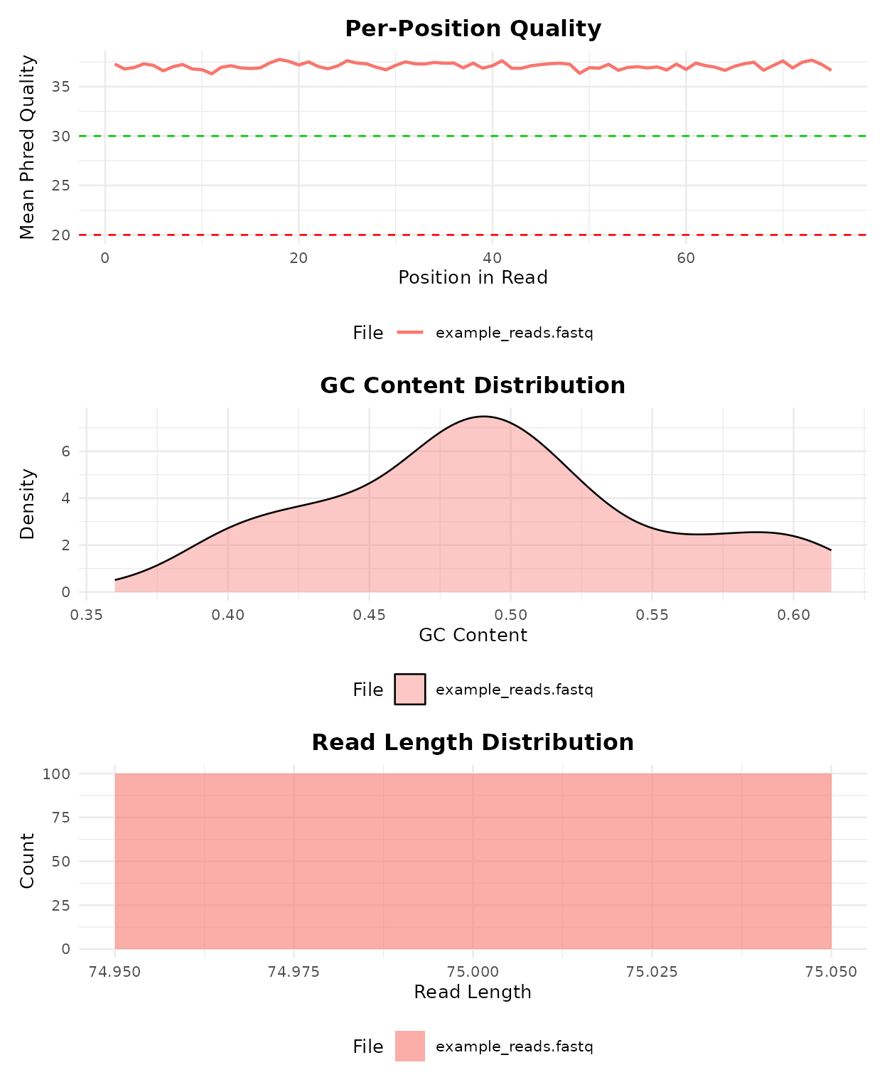

QC visualization panel: per-position quality, GC content, and read length distribution.

Differential Expression

Three DE methods are supported, each requiring an optional Bioconductor package. All three return a standardized data.frame with columns gene, log2fc, pvalue, padj, and optionally basemean.

# DESeq2 (requires DESeq2)
de <- bb_deseq2(counts, metadata)

# edgeR (requires edgeR)
de <- bb_edger(counts, group = metadata$condition)

# limma-voom (requires limma + edgeR)
design <- model.matrix(~ condition, data = metadata)
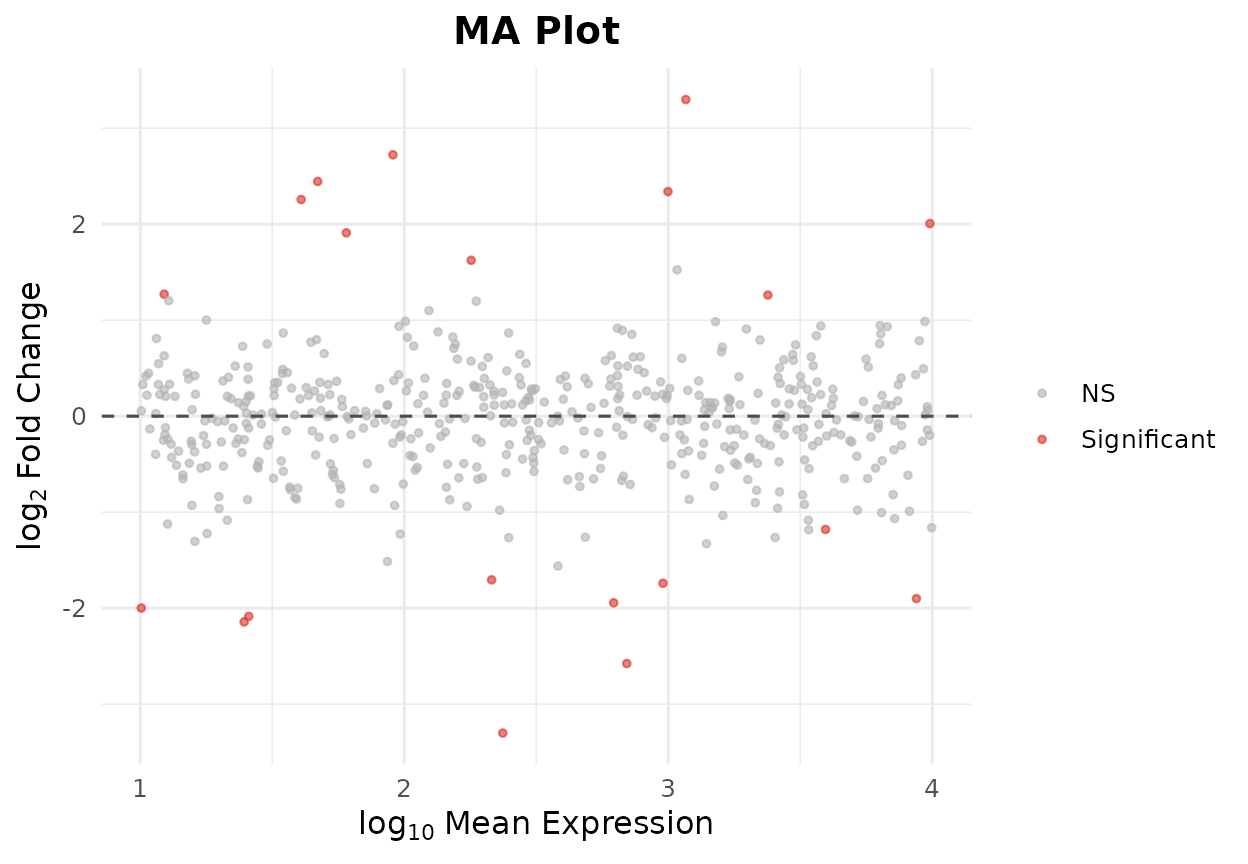
de <- bb_limma_voom(counts, design)

The standardized output ensures that bb_volcano(), bb_ma_plot(), bb_heatmap(), and bb_export_csv() work identically regardless of the DE method used.

Export

bb_export_csv(de_results, "de_results.csv")
bb_export_tsv(de_results, "de_results.tsv")
bb_export_rds(de_results, "de_results.rds")

Full Pipeline

The bb_pipeline() function runs the entire analysis end-to-end. It accepts entry at three stages:

# From FASTQ files
result <- bb_pipeline(
  fastq_dir    = "raw_reads/",
  genome_index = "STAR_index/",
  annotation   = "genes.gtf",
  sample_info  = metadata,
  aligner      = "STAR",
  de_method    = "DESeq2",
  threads      = 8
)

# From BAM files (skip alignment)
result <- bb_pipeline(
  bam_dir     = "aligned/",
  annotation  = "genes.gtf",
  sample_info = metadata
)

# From a count matrix (skip alignment + counting)
result <- bb_pipeline(
  count_matrix = my_counts,
  sample_info  = metadata,
  de_method    = "edgeR"
)

The returned bb_result object bundles counts, metadata, DE results, and all generated plots:

result$counts          # count matrix
result$de_results      # standardized DE data.frame
result$plots$pca       # ggplot object
result$plots$volcano   # ggplot object
result$plots$heatmap   # ggplot object

Interactive Shiny App

Launch a browser-based dashboard for interactive analysis:

bb_run_app()

The app provides:

Data upload (CSV, TSV, RDS) with live preview
Configurable normalization and DE parameters
Interactive plots (volcano, PCA, heatmap, MA, oncoplot)
One-click export (CSV, RDS, PDF)

Function Reference

Import

Function	Description
`bb_read_fastq()`	Read FASTQ files
`bb_read_bam()`	Read BAM files
`bb_count_bam()`	Count reads in BAM

Quality Control

Function	Description
`bb_qc()`	Compute QC metrics
`bb_qc_summary()`	Tabular QC summary
`bb_plot_qc()`	QC visualization panel

Alignment & Counting

Function	Description
`bb_align()`	Align with STAR / HISAT2 / minimap2
`bb_count_reads()`	Count reads per gene

Normalization

Function	Description
`bb_normalize()`	CPM, TPM, TMM, or RLE

Differential Expression

Function	Description
`bb_deseq2()`	DESeq2 wrapper
`bb_edger()`	edgeR quasi-likelihood wrapper
`bb_limma_voom()`	limma-voom wrapper

Visualization

Function	Description
`bb_oncoplot()`	Waterfall mutation plot
`bb_volcano()`	Volcano plot
`bb_heatmap()`	Clustered heatmap
`bb_pca()`	PCA plot
`bb_ma_plot()`	MA plot

Pipeline & Export

Function	Description
`bb_pipeline()`	Full end-to-end pipeline
`bb_export_csv()`	Export as CSV
`bb_export_tsv()`	Export as TSV
`bb_export_rds()`	Export as RDS

Example Data & App

Function	Description
`bb_example_counts()`	Example count matrix
`bb_example_mutations()`	Example mutation data
`bb_example_de()`	Example DE results
`bb_run_app()`	Launch Shiny dashboard

Citation

If you use bambamR in your research, please cite:

Heller R, Witte H, Steinestel K (2026). bambamR: End-to-End RNA-Seq Processing from FASTQ to Publication-Ready Plots. R package version 0.1.0. https://github.com/r-heller/bambamR

Session Info

sessionInfo()
#> R version 4.6.0 (2026-04-24)
#> Platform: x86_64-pc-linux-gnu
#> Running under: Ubuntu 24.04.4 LTS
#> 
#> Matrix products: default
#> BLAS:   /usr/lib/x86_64-linux-gnu/openblas-pthread/libblas.so.3 
#> LAPACK: /usr/lib/x86_64-linux-gnu/openblas-pthread/libopenblasp-r0.3.26.so;  LAPACK version 3.12.0
#> 
#> locale:
#>  [1] LC_CTYPE=C.UTF-8       LC_NUMERIC=C           LC_TIME=C.UTF-8       
#>  [4] LC_COLLATE=C.UTF-8     LC_MONETARY=C.UTF-8    LC_MESSAGES=C.UTF-8   
#>  [7] LC_PAPER=C.UTF-8       LC_NAME=C              LC_ADDRESS=C          
#> [10] LC_TELEPHONE=C         LC_MEASUREMENT=C.UTF-8 LC_IDENTIFICATION=C   
#> 
#> time zone: UTC
#> tzcode source: system (glibc)
#> 
#> attached base packages:
#> [1] stats     graphics  grDevices utils     datasets  methods   base     
#> 
#> other attached packages:
#> [1] bambamR_0.1.0
#> 
#> loaded via a namespace (and not attached):
#>  [1] farver_2.1.2                Biostrings_2.80.0          
#>  [3] S7_0.2.2                    bitops_1.0-9               
#>  [5] fastmap_1.2.0               GenomicAlignments_1.48.0   
#>  [7] digest_0.6.39               lifecycle_1.0.5            
#>  [9] pwalign_1.8.0               cluster_2.1.8.2            
#> [11] statmod_1.5.1               compiler_4.6.0             
#> [13] rlang_1.2.0                 sass_0.4.10                
#> [15] tools_4.6.0                 yaml_2.3.12                
#> [17] knitr_1.51                  S4Arrays_1.12.0            
#> [19] labeling_0.4.3              htmlwidgets_1.6.4          
#> [21] interp_1.1-6                DelayedArray_0.38.1        
#> [23] RColorBrewer_1.1-3          ShortRead_1.70.0           
#> [25] abind_1.4-8                 BiocParallel_1.46.0        
#> [27] withr_3.0.2                 hwriter_1.3.2.1            
#> [29] BiocGenerics_0.58.0         desc_1.4.3                 
#> [31] grid_4.6.0                  stats4_4.6.0               
#> [33] latticeExtra_0.6-31         colorspace_2.1-2           
#> [35] edgeR_4.10.0                ggplot2_4.0.3              
#> [37] scales_1.4.0                iterators_1.0.14           
#> [39] SummarizedExperiment_1.42.0 cli_3.6.6                  
#> [41] rmarkdown_2.31              crayon_1.5.3               
#> [43] ragg_1.5.2                  generics_0.1.4             
#> [45] otel_0.2.0                  rjson_0.2.23               
#> [47] cachem_1.1.0                parallel_4.6.0             
#> [49] XVector_0.52.0              matrixStats_1.5.0          
#> [51] vctrs_0.7.3                 Matrix_1.7-5               
#> [53] jsonlite_2.0.0              IRanges_2.46.0             
#> [55] GetoptLong_1.1.1            patchwork_1.3.2            
#> [57] S4Vectors_0.50.0            ggrepel_0.9.8              
#> [59] clue_0.3-68                 systemfonts_1.3.2          
#> [61] jpeg_0.1-11                 locfit_1.5-9.12            
#> [63] foreach_1.5.2               limma_3.68.1               
#> [65] jquerylib_0.1.4             glue_1.8.1                 
#> [67] pkgdown_2.2.0               codetools_0.2-20           
#> [69] gtable_0.3.6                shape_1.4.6.1              
#> [71] deldir_2.0-4                GenomicRanges_1.64.0       
#> [73] ComplexHeatmap_2.28.0       htmltools_0.5.9            
#> [75] Seqinfo_1.2.0               circlize_0.4.18            
#> [77] R6_2.6.1                    textshaping_1.0.5          
#> [79] doParallel_1.0.17           evaluate_1.0.5             
#> [81] lattice_0.22-9              Biobase_2.72.0             
#> [83] png_0.1-9                   Rsamtools_2.28.0           
#> [85] cigarillo_1.2.0             bslib_0.10.0               
#> [87] Rcpp_1.1.1-1.1              SparseArray_1.12.2         
#> [89] DESeq2_1.52.0               xfun_0.57                  
#> [91] fs_2.1.0                    MatrixGenerics_1.24.0      
#> [93] GlobalOptions_0.1.4

Raban Heller, Hanno Witte, Konrad Steinestel — BwKrhs Ulm

2026-05-04

Introduction

Key Design Principles

Minimal vs. Full Mode

Installation

Bundled Example Data

Normalization

CPM (Counts Per Million)

TPM (Transcripts Per Million)

TMM and RLE (Bioconductor)

Visualization

PCA Plot

Heatmap

Volcano Plot

MA Plot

Heatmap of Top DE Genes

Oncoplot

Data Format

Basic Oncoplot

Oncoplot with Clinical Annotations

Selecting Specific Genes

Custom Colors

FASTQ Import

Quality Control

Differential Expression

Export

Full Pipeline

Interactive Shiny App

Function Reference

Import

Quality Control

Alignment & Counting

Normalization

Differential Expression

Visualization

Pipeline & Export

Example Data & App

Citation

Session Info