library(ggplot2)Lab W1 · Counting people, images and readings
Teaching units 02–04: twelve synthetic register rows with a repeated identifier and a unit error, a data dictionary, a fixed rule against a learnt threshold, and a reduced teaching table.
This is the first R lab of the course. You need only four things: a table (data.frame), a count (nrow(), length(unique())), a selection with square brackets and one figure. Read each chunk, predict what it will print, then compare. Every part follows the same five steps: decision, look at the data, assumption, compute, report.
TipStarting R for the first time
Open the script in RStudio or Positron and run it line by line (Ctrl/Cmd + Enter). If installation fails, work with the printed output on this page and a partner’s computer; the paper version of the tasks is the same.
Part A · How many observations are in twelve rows? (unit 02)
Decision. A study team wants to know how many patients with a wrist injury had a fracture read on imaging. The register export below has twelve rows. Before anyone computes a percentage, the team must agree on the denominator.
Look at the data. Count by hand first: how many people, how many images, how many readings? Write your three numbers down.
# Twelve rows as exported from a fictitious wrist-injury register (synthetic)
raw <- data.frame(
  row         = 1:12,
  person_id   = c("P01", "P01", "P01", "P02", "P02", "P3", "P03", "P04", "P04", "P04", "P05", "P05"),
  image_id    = c("P01-A", "P01-A", "P01-B", "P02-A", "P02-A", "P03-A", "P03-A", "P04-A", "P04-B", "P04-B",
                  "P05-A", "P05-A"),
  reader      = c("radiology", "emergency", "radiology", "radiology", "emergency", "radiology", "emergency",
                  "radiology", "radiology", "emergency", "radiology", "emergency"),
  fracture_read = c("yes", "yes", "yes", "no", "yes", "no", "no", "yes", "yes", "yes", "no", "no"),
  wrist_cm    = c(18.2, 18.2, 18.0, 16.1, 16.1, 17.4, 174, 19.0, 18.6, 18.6, 15.8, 15.8),
  age_years   = c(34, 34, 34, 71, 71, 52, 52, 88, 88, 88, 23, 23),
  hours_since_injury = c(2, 2, 50, 5, 5, 1, 1, 26, 74, 74, 3, 3),
  free_text   = c("cyclist, fell on the way to the bakery she owns", "", "follow-up image", "",
                  "lives alone, daughter is a nurse on ward 4", "", "", "fall in care home, room 12", "", "",
                  "goalkeeper, regional league", "")
)
raw[, c("row", "person_id", "image_id", "reader", "fracture_read", "wrist_cm")]
#> row person_id image_id reader fracture_read wrist_cm
#> 1 1 P01 P01-A radiology yes 18.2
#> 2 2 P01 P01-A emergency yes 18.2
#> 3 3 P01 P01-B radiology yes 18.0
#> 4 4 P02 P02-A radiology no 16.1
#> 5 5 P02 P02-A emergency yes 16.1
#> 6 6 P3 P03-A radiology no 17.4
#> 7 7 P03 P03-A emergency no 174.0
#> 8 8 P04 P04-A radiology yes 19.0
#> 9 9 P04 P04-B radiology yes 18.6
#> 10 10 P04 P04-B emergency yes 18.6
#> 11 11 P05 P05-A radiology no 15.8
#> 12 12 P05 P05-A emergency no 15.8Now let R count every distinct entry without thinking:
# Counting without looking: every row, every distinct text in person_id and image_id
c(rows = nrow(raw), persons = length(unique(raw$person_id)), images = length(unique(raw$image_id)))
#> rows persons images
#> 12 6 7Assumption. Rows are readings, not people. An identifier means the same thing in every row. Both assumptions fail here in different ways. Look for the identifier error and for a value in the wrong unit:
# 1. Identifier error: the same person written as "P3" and "P03"
sort(unique(raw$person_id))
#> [1] "P01" "P02" "P03" "P04" "P05" "P3"# 2. Unit error: wrist circumference outside a plausible adult range (12 to 30 cm)
raw[raw$wrist_cm < 12 | raw$wrist_cm > 30, c("row", "person_id", "wrist_cm")]#> row person_id wrist_cm
#> 7 7 P03 174# Corrected copy: identifiers padded to two digits, the value in millimetres converted to centimetres
clean <- raw
clean$person_id <- sprintf("P%02d", as.integer(sub("^P", "", clean$person_id)))
clean$wrist_cm[clean$wrist_cm > 30] <- clean$wrist_cm[clean$wrist_cm > 30] / 10
counts <- c(rows = nrow(clean), persons = length(unique(clean$person_id)),
images = length(unique(clean$image_id)))
counts#> rows persons images
#> 12 5 7# Target values: 12 readings of 7 images from 5 people; the unit error is in row 7
stopifnot(counts[["rows"]] == 12, counts[["persons"]] == 5, counts[["images"]] == 7,
length(unique(raw$person_id)) == 6, which(raw$wrist_cm > 30) == 7,
all(clean$wrist_cm >= 12 & clean$wrist_cm <= 30))Report. The export holds 12 readings of 7 images from 5 people. For a question about patients, the independent unit is the person; counting rows would inflate the denominator by more than a factor of two. Row 7 records the wrist circumference in millimetres instead of centimetres.
plot_data <- clean
plot_data$reader <- factor(plot_data$reader, levels = c("radiology", "emergency"))
p_units <- ggplot(plot_data, aes(x = person_id, y = image_id, shape = reader, colour = fracture_read)) +
  geom_point(size = 3.5, position = position_nudge(x = ifelse(plot_data$reader == "radiology", -0.12, 0.12))) +
  scale_colour_manual(values = c(yes = unname(cdsr_colours["red"]), no = unname(cdsr_colours["blue"]))) +
  scale_shape_manual(values = cdsr_shapes[1:2]) +
  labs(x = "Person (corrected identifier)", y = "Image", shape = "Reader", colour = "Fracture read",
       caption = "Synthetic register extract: 12 readings of 7 images from 5 people.") +
  theme_cdsr()
show_figure(p_units, "w1-units.png", height = 4)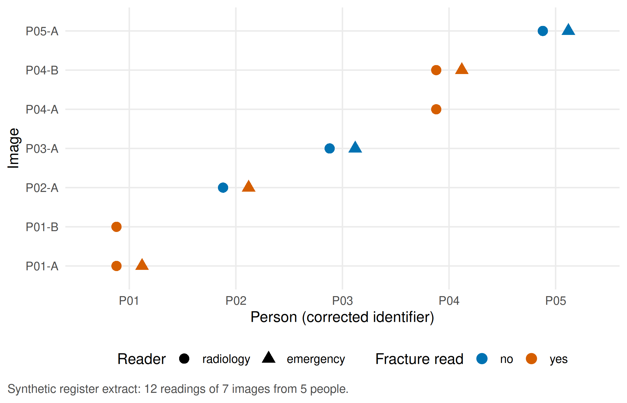
Two readers disagree on one image:
# Readings per image and agreement between readers on the same image
per_image <- aggregate(fracture_read ~ image_id, data = clean,
                       FUN = function(x) paste(x, collapse = "/"))
per_image$readings <- as.vector(table(clean$image_id)[per_image$image_id])
per_image$agree <- !grepl("yes", per_image$fracture_read) | !grepl("no", per_image$fracture_read)
per_image
#> image_id fracture_read readings agree
#> 1 P01-A yes/yes 2 TRUE
#> 2 P01-B yes 1 TRUE
#> 3 P02-A no/yes 2 FALSE
#> 4 P03-A no/no 2 TRUE
#> 5 P04-A yes 1 TRUE
#> 6 P04-B yes/yes 2 TRUE
#> 7 P05-A no/no 2 TRUEstopifnot(sum(!per_image$agree) == 1, per_image$image_id[!per_image$agree] == "P02-A")
TipCounter-check: predict first
Suppose the team reports “fracture read in 7 of 12 cases”. Which denominator is that, and what would the statement be at image level and at person level? Decide how you count a person whose two readers disagree before you look at the table again.
Part B · A data dictionary (unit 02)
Decision. Which columns may leave the clinical system for a teaching or research table, and what does each column mean?
A data dictionary names, for every column, its meaning, its unit, its time zero and the reason it was collected. Time zero matters: “hours since injury” starts at a self-reported moment, “wrist circumference” at the time of imaging.
# Data dictionary: key, unit, time zero and reason for collection for every column
dictionary <- data.frame(
  column = names(clean),
  meaning = c("row number of the export", "person identifier (key for person-level questions)",
              "image identifier (key for image-level questions)", "who read the image",
              "reader's judgement: fracture yes/no", "wrist circumference of the injured side",
              "age at presentation", "time from injury to imaging", "free-text note"),
  unit = c("-", "-", "-", "-", "-", "cm", "years", "hours", "-"),
  time_zero = c("-", "-", "-", "-", "time of reading", "time of imaging", "presentation",
                "injury (self-reported)", "-"),
  collected_for = c("export", "care", "care", "care", "care", "care", "care", "care", "care"),
  needed_for_teaching = c("no", "yes (pseudonym)", "yes (pseudonym)", "yes", "yes", "yes", "yes", "yes", "no")
)
dictionary
#> column meaning unit
#> 1 row row number of the export -
#> 2 person_id person identifier (key for person-level questions) -
#> 3 image_id image identifier (key for image-level questions) -
#> 4 reader who read the image -
#> 5 fracture_read reader's judgement: fracture yes/no -
#> 6 wrist_cm wrist circumference of the injured side cm
#> 7 age_years age at presentation years
#> 8 hours_since_injury time from injury to imaging hours
#> 9 free_text free-text note -
#> time_zero collected_for needed_for_teaching
#> 1 - export no
#> 2 - care yes (pseudonym)
#> 3 - care yes (pseudonym)
#> 4 - care yes
#> 5 time of reading care yes
#> 6 time of imaging care yes
#> 7 presentation care yes
#> 8 injury (self-reported) care yes
#> 9 - care noReport. Two columns are not needed for any teaching question: the export row number and the free-text note. The free text contains details that can identify a person on their own (an occupation, a care-home room, a relative’s ward).
Part C · A fixed rule against a learnt threshold (unit 03)
Decision. Should a simple alert use a cut-off written down in advance or one learnt from data?
Look at the data. For 60 synthetic people we know the difference in wrist circumference between the injured and the uninjured side and whether a fracture was present. The first 40 people are the training data, the remaining 20 the application data. Nobody appears in both.
Assumption. The rule (“alert at a difference of 1.0 cm or more”) was fixed before seeing any data. The learnt threshold is the cut-off that best separates fractures from non-fractures in the 40 training people.
# Part C (unit 03): a fixed rule against a threshold learnt from training data (60 synthetic people)
set.seed(12)
m <- 60
swell <- data.frame(person_id = sprintf("S%02d", 1:m), fracture = rbinom(m, 1, 0.35))
# difference in wrist circumference, injured minus uninjured side, in cm (synthetic)
swell$diff_cm <- round(rnorm(m, mean = ifelse(swell$fracture == 1, 1.7, 0.6), sd = 0.65), 1)
swell$phase <- ifelse(seq_len(m) <= 40, "training", "application")
train <- swell[swell$phase == "training", ]
apply_set <- swell[swell$phase == "application", ]

# Rule: written down before seeing any data
rule_cm <- 1.0
# Learnt threshold: the cut-off that maximises sensitivity + specificity in the training people
candidates <- sort(unique(train$diff_cm))
youden <- sapply(candidates, function(t) {
  mean(train$diff_cm[train$fracture == 1] >= t) + mean(train$diff_cm[train$fracture == 0] < t) - 1
})
learnt_cm <- candidates[which.max(youden)]

evaluate <- function(threshold, d) {
  alert <- d$diff_cm >= threshold
  c(threshold = threshold, alerts = sum(alert), detected = sum(alert & d$fracture == 1),
    fractures = sum(d$fracture == 1), false_alerts = sum(alert & d$fracture == 0))
}
comparison <- rbind(rule = evaluate(rule_cm, apply_set), learnt = evaluate(learnt_cm, apply_set))
comparison
#> threshold alerts detected fractures false_alerts
#> rule 1.0 7 5 5 2
#> learnt 1.3 6 4 5 2stopifnot(nrow(train) == 40, nrow(apply_set) == 20,
length(intersect(train$person_id, apply_set$person_id)) == 0,
learnt_cm == 1.3,
all(comparison["rule", c("alerts", "detected", "fractures", "false_alerts")] == c(7, 5, 5, 2)),
all(comparison["learnt", c("alerts", "detected", "fractures", "false_alerts")] == c(6, 4, 5, 2)))p_thr <- ggplot(train, aes(x = diff_cm, y = factor(fracture, labels = c("no fracture", "fracture")))) +
geom_point(position = position_jitter(height = 0.12, width = 0, seed = 1),
colour = cdsr_colours[["blue"]], shape = cdsr_shapes[1], size = 2.2) +
geom_vline(xintercept = rule_cm, linetype = cdsr_linetypes[2], colour = cdsr_colours[["grey"]]) +
geom_vline(xintercept = learnt_cm, linetype = cdsr_linetypes[1], colour = cdsr_colours[["orange"]]) +
annotate("text", x = rule_cm, y = 2.45, label = "rule", hjust = 1.1, colour = cdsr_colours[["grey"]]) +
annotate("text", x = learnt_cm, y = 2.45, label = "learnt", hjust = -0.1, colour = cdsr_colours[["orange"]]) +
labs(x = "Difference in wrist circumference, injured minus uninjured side (cm)", y = NULL,
caption = "Synthetic training data, n = 40 people. Dashed line: fixed rule; solid line: learnt threshold.") +
theme_cdsr()
show_figure(p_thr, "w1-threshold.png", height = 3.6)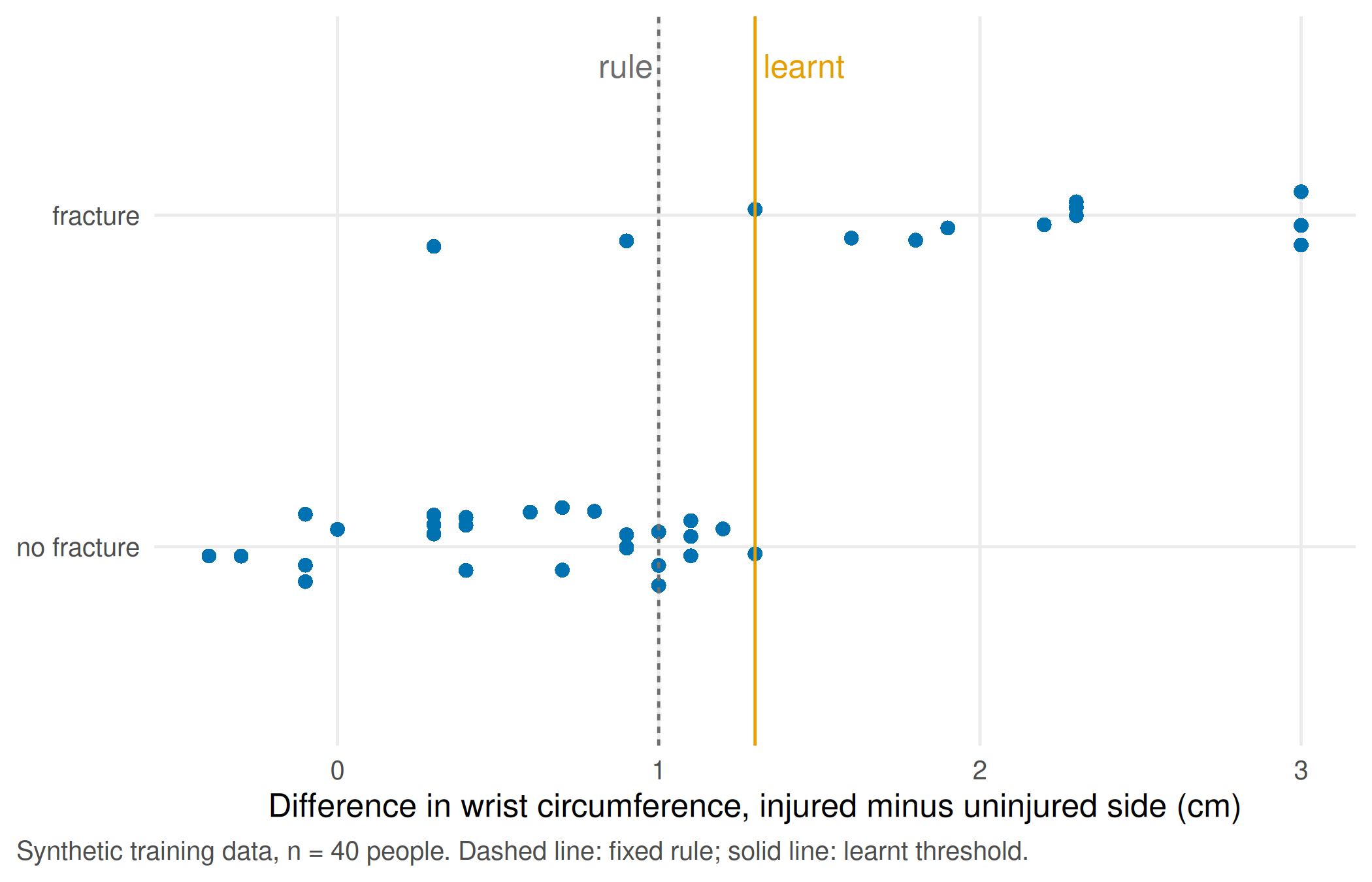
Report. In the 20 application people, the fixed rule raises 7 alerts and finds 5 of 5 fractures; the learnt threshold of 1.3 cm raises 6 alerts and finds 4. “Learning” here means nothing more than choosing a number from training data; with 40 people that number is unstable, as the counter-check shows.
TipCounter-check: predict first
The threshold is learnt again from a different set of 40 people drawn from the same 60. Will it stay at 1.3 cm, move by about 0.1 cm, or move by more? Then run the chunk.
# Counter-check: learn the threshold again from a different set of 40 training people
set.seed(7)
other_train <- swell[sample(m, 40), ]
cand2 <- sort(unique(other_train$diff_cm))
learnt_again <- cand2[which.max(sapply(cand2, function(t) {
  mean(other_train$diff_cm[other_train$fracture == 1] >= t) +
    mean(other_train$diff_cm[other_train$fracture == 0] < t) - 1
}))]
c(first = learnt_cm, second = learnt_again)
#> first second
#> 1.3 1.6stopifnot(learnt_again == 1.6)Part D · A reduced teaching table (unit 04)
Decision. The table will be used in a course. What is the smallest table that still answers the teaching questions?
Assumption. Pseudonymised identifiers stay (they are needed to count people and images); the free text and the exact age go; age is kept in four bands. Whether such a table may be shared outside the clinic is a separate question of data protection and local approval (open; see W7).
# Part D (unit 04): the reduced teaching table keeps only what the exercise needs
teaching <- clean[, c("person_id", "image_id", "reader", "fracture_read", "wrist_cm", "age_years",
                      "hours_since_injury")]
teaching$age_group <- cut(teaching$age_years, c(17, 39, 64, 79, 120),
                          labels = c("18-39", "40-64", "65-79", "80+"))
teaching$age_years <- NULL                       # exact age not needed for the exercise
stopifnot(!"free_text" %in% names(teaching), !"age_years" %in% names(teaching), nrow(teaching) == 12)
teaching
#> person_id image_id reader fracture_read wrist_cm hours_since_injury
#> 1 P01 P01-A radiology yes 18.2 2
#> 2 P01 P01-A emergency yes 18.2 2
#> 3 P01 P01-B radiology yes 18.0 50
#> 4 P02 P02-A radiology no 16.1 5
#> 5 P02 P02-A emergency yes 16.1 5
#> 6 P03 P03-A radiology no 17.4 1
#> 7 P03 P03-A emergency no 17.4 1
#> 8 P04 P04-A radiology yes 19.0 26
#> 9 P04 P04-B radiology yes 18.6 74
#> 10 P04 P04-B emergency yes 18.6 74
#> 11 P05 P05-A radiology no 15.8 3
#> 12 P05 P05-A emergency no 15.8 3
#> age_group
#> 1 18-39
#> 2 18-39
#> 3 18-39
#> 4 65-79
#> 5 65-79
#> 6 40-64
#> 7 40-64
#> 8 80+
#> 9 80+
#> 10 80+
#> 11 18-39
#> 12 18-39Report. The teaching table has 12 rows and no free text or exact age. Every removed column is listed in the data dictionary with the reason it is not needed.
Your record for the workshop
- The three counts (readings, images, people) with the error you found in each.
- The data dictionary with key, unit, time zero and reason for collection.
- A sketch of rule versus learnt threshold, marking which data were used for training and which for application, and the script that recreates the table in a fresh R session.
- The reduced teaching table and one sentence justifying each removed field.
Further reading
- Companion book: B01 · Clinical decisions and the translational chain and B03 · How data arise: missingness and denominators – why the denominator is a clinical decision.
- B04 · Reconstructing a research project in R – scripts, relative paths and a target value that a colleague can check.
- CTTIR Courses: Data types, tidy data, accuracy and precision – long and wide tables, one row per observation.
- CTTIR Courses: Import, joins, and missingness with dplyr – the next step after base R.
- Methods in R: Scales of Measurement – units and measurement levels.