4  Reconstructing a research project in R

Author

R. Heller

R. Heller · Date: 2026-06-28 · Last changed: 2026-11-09

NoteAt a glance

Guiding question: Can a colleague regenerate the number in the figure?

For: anyone who hands over, reviews or reuses an analysis; readers taking their first steps in R · Prerequisites: Chapter 3 (the fracture cohort tables); the Lab of Chapter 1

In the course: W1 · From clinical case to question (a script that rebuilds the table in a fresh session), W6 · Pharmacometrics, forecasting and simulation (another group checks one number) and W8 · Colloquium and decision; recommended reading · Data: synthetic (built in the chapter; compared with b03-visits.csv) · Core reading time: about 10 minutes

4.1 Case and decision

Six months after the board meeting in Chapter 3, a fictional rehabilitation physician is asked to include one number in a grant report: mean gait speed 0.56 m/s in weeks three to five after surgery, n = 7 of 12 patients. She asks the physiotherapy team to regenerate it. They find a spreadsheet called final_v3_corrected.xlsx, a figure pasted into a slide and no script. A colleague remembers that the sensor-mat values were “divided by 100 somewhere”, that one patient identifier was fixed by hand and that a duplicate row was deleted. Nobody can say in which order, or whether anything else happened. The physician has to decide whether the number may go into the report. The department decides on a rule for the future: a number leaves the team only if one command can regenerate it from the raw exports.

4.2 Core reading

Core reading · recommended for W1, W6 and W8 · about 10 minutes · ends before ‘Lab’

4.2.1 Reproducible is a modest, checkable promise

A result is reproducible when the same data and the same code produce the same number. This is less than replication, which asks whether new data lead to the same conclusion. Peng described reproducibility as the minimum standard for judging a computational claim when full replication is not possible (Peng 2011). It is modest because it says nothing about whether the analysis is right. It is valuable because anyone can check it, and because every error that is found can be traced to a line of code.

The spreadsheet in the case fails this standard not because spreadsheets are bad, but because the steps that changed the data were performed by hand and left no trace. Such hidden interactive steps are common: editing cells, filtering in a viewer and copying the visible rows, retyping a number from one window into another. Some are not even chosen by the user. Ziemann and colleagues found that about one-fifth of genomics papers with supplementary Excel gene lists contained gene names that the software had silently converted into dates or numbers (published) (Ziemann et al. 2016).

Sandve and colleagues condensed the remedy into ten rules (Sandve et al. 2013). Five of them carry this chapter: keep track of how every result was produced; avoid manual data manipulation; archive the exact versions of the software used; put all custom scripts under version control; and, for analyses with randomness, record the seed.

4.2.2 A project that runs with one command

Wilson and colleagues describe “good enough” practices for researchers without formal training in programming (Wilson et al. 2017). Applied to the fracture cohort, they lead to a small folder structure:

hip-gait-project/
├── README.md               start instructions, data schema, target value
├── ARTEFACTS.csv           provenance, rights and data status of every exported file
├── run.R                   the one command:  Rscript run.R
├── R/                      code, numbered in the order it runs
│   ├── 00_visits.R         planned-visit table of chapter B03 (synthetic)
│   ├── 01_simulate_raw.R   raw exports (in a real project: delivered, read-only)
│   ├── 02_clean.R          documented cleaning instead of manual edits
│   ├── 03_check.R          counts on two independent paths
│   └── 04_figure.R         figure and target value
├── data/raw/               written once, never edited
├── data/derived/           always regenerated, never edited by hand
├── output/                 figure, session information
└── report/report.qmd       Quarto report: text and numbers from the same code

Three conventions do most of the work. First, raw data are read-only; every change happens in code. Second, every path is relative to the project folder, such as data/raw/sensormat.csv, never C:/Users/anna/Desktop/..., so the folder runs on any computer. Third, the project states a target value, a number that must come out, and stops with an error if it does not. Here it is the number from the case: in visit window V4, 7 of 12 patients measured, mean gait speed 0.56 m/s.

4.2.3 What a colleague needs to rerun it

A colleague who receives the folder should not need to ask anything. The README answers four questions in this order: how to start (one command), what the input files contain (the data schema: one line per file with its unit of observation, its key and the unit of every measured column), which number must come out (the target value), and under which terms the files may be used. The data schema is where the case went wrong: the stopwatch export gives seconds for four metres, the sensor mat gives centimetres per second, and only the conversion written in code makes both comparable. The second safeguard is the count on two paths, as in Chapter 3. Patients, measurements and linked records are computed once from the visit table and once from the patient table with different functions; any lost or duplicated row shows up as a disagreement. Both checks are cheap, and both fail loudly instead of producing a plausible figure.

4.2.4 Versions of code, data and software

A project changes over time. Git, a version control system, records every change to text files with author, date and a short message, so that the state of the code on the day a figure was made can be restored (Bryan 2018). The R function sessionInfo() records the versions of R and of every loaded package; it belongs in every report. Quarto turns a text file with embedded R code into a report in which every number in the text is computed, not typed (Quarto, n.d.). Text and figure can then no longer drift apart.

4.2.5 Every exported file carries its passport

Files travel: into slides, e-mails, other projects. Once they leave the project folder, they lose their context. Each exported artefact therefore needs three pieces of information that travel with it: its provenance (which code made it from which input), its rights (who may use it under which licence) and its data status (synthetic, published, real and pseudonymised, aggregate). Table 4.1 shows them for the project in this chapter.

Table 4.1: Provenance, rights and data status of every exported artefact of the teaching project (n = 12 synthetic patients). In a project with real data, the rights column would name the data use agreement and ethics approval, and the raw files would not be released.
Artefact Produced by Provenance Rights Data status
data/raw/*.csv (4 files) R/01_simulate_raw.R Generated from the planned-visit table of Chapter 3 CC BY 4.0 synthetic
data/derived/visits.csv R/02_clean.R From the four raw files; cleaning log: 1 duplicate removed, 1 identifier corrected CC BY 4.0 synthetic
output/figure-windows.png R/04_figure.R From data/derived/visits.csv CC BY 4.0 synthetic, aggregate
output/session-info.txt run.R Software versions of the run CC BY 4.0 technical metadata
report/report.html Quarto, report/report.qmd Text, figure and numbers from the files above Text CC BY 4.0; code MIT synthetic, aggregate
R/*.R, run.R Authors — MIT code, no data

A number counts as reproduced only if code alone regenerates it from the raw exports in a fresh R session and it matches the stated target value. A number that is retyped or copied counts as unreproduced, however plausible it looks.

Question for the workshop: Give your script and raw files to another group. They start a fresh R session, run one command and report the target value. Which file, package or step did they need that was not in your project?

4.3 Lab

4.3.1 Step 1: R objects in five minutes

R works with objects that have a name. The most important are vectors (a sequence of values of one type) and data frames (several vectors of equal length side by side). Ms K.’s five gait-speed values from Chapter 3 serve as example.

gait <- c(0.31, 0.42, 0.55, 0.63, 0.78)    # numeric vector, metres per second
day  <- c(2, 6, 15, 27, 91)                 # days since surgery
length(gait)                                # how many values
#> [1] 5
mean(gait)                                  # one number from five
#> [1] 0.538
gait[day > 10]                              # values after day 10: logical selection with [ ]
#> [1] 0.55 0.63 0.78
class(gait)                                 # the type of the object
#> [1] "numeric"
with_gap <- c(0.31, NA, 0.55)               # NA = not available
mean(with_gap)                              # NA is contagious ...
#> [1] NA
mean(with_gap, na.rm = TRUE)                # ... unless it is removed on purpose
#> [1] 0.43

The last two lines are the whole of Chapter 3 in miniature: R refuses to average over a missing value until you tell it to, and from then on the denominator is smaller without anyone seeing it.

4.3.2 Step 2: reading a file with a relative path

The planned-visit table was saved by Chapter 3 in the book’s data folder. This chapter lives in the chapters folder, so the relative path goes one level up (..) and then into data.

path_b03 <- file.path("..", "data", "b03-visits.csv")
stopifnot(file.exists(path_b03))
visits_b03 <- read.csv(path_b03, stringsAsFactors = FALSE)
str(visits_b03)
#> 'data.frame':    60 obs. of  6 variables:
#>  $ pid    : chr  "P01" "P01" "P01" "P01" ...
#>  $ window : chr  "V1" "V2" "V3" "V4" ...
#>  $ day    : int  2 6 15 27 91 1 5 13 29 88 ...
#>  $ gait_ms: num  0.31 0.42 0.55 0.63 0.78 0.28 0.35 0.47 0.58 0.7 ...
#>  $ status : chr  "measured" "measured" "measured" "measured" ...
#>  $ method : chr  "stopwatch" "stopwatch" "sensor mat" "sensor mat" ...

str() shows the structure: 60 rows (observations), 6 columns (variables), the type of each column (chr for text, int or num for numbers) and the first values. Missing values appear as NA. If R reports “cannot open file”, the working directory is not the folder you think; getwd() shows where R is looking.

4.3.3 Step 3: a base graphic

Base R draws graphics without additional packages. cdsr_par() sets the book’s margins and fonts; plot() draws points and lines; text() writes labels at given coordinates. The function below is the figure of the project, and it is used again in Step 7.

summarise_windows <- function(visits) {
  data.frame(window  = sort(unique(visits$window)),
             n       = as.vector(tapply(visits$status == "measured", visits$window, sum)),
             of      = as.vector(table(visits$window)),
             mean_ms = as.vector(tapply(visits$gait_ms, visits$window, mean, na.rm = TRUE)))
}
draw_windows <- function(s) {
  plot(seq_len(nrow(s)), s$mean_ms, type = "b", pch = 16, ylim = c(0, 1), xlim = c(0.5, nrow(s) + 0.5), xaxt = "n",
       xlab = "Planned visit window", ylab = "Mean gait speed (m/s)")
  axis(1, at = seq_len(nrow(s)), labels = s$window)
  text(seq_len(nrow(s)), s$mean_ms, paste0("n = ", s$n, "/", s$of), pos = 3, cex = 0.85)
}
cdsr_par()
draw_windows(summarise_windows(visits_b03))
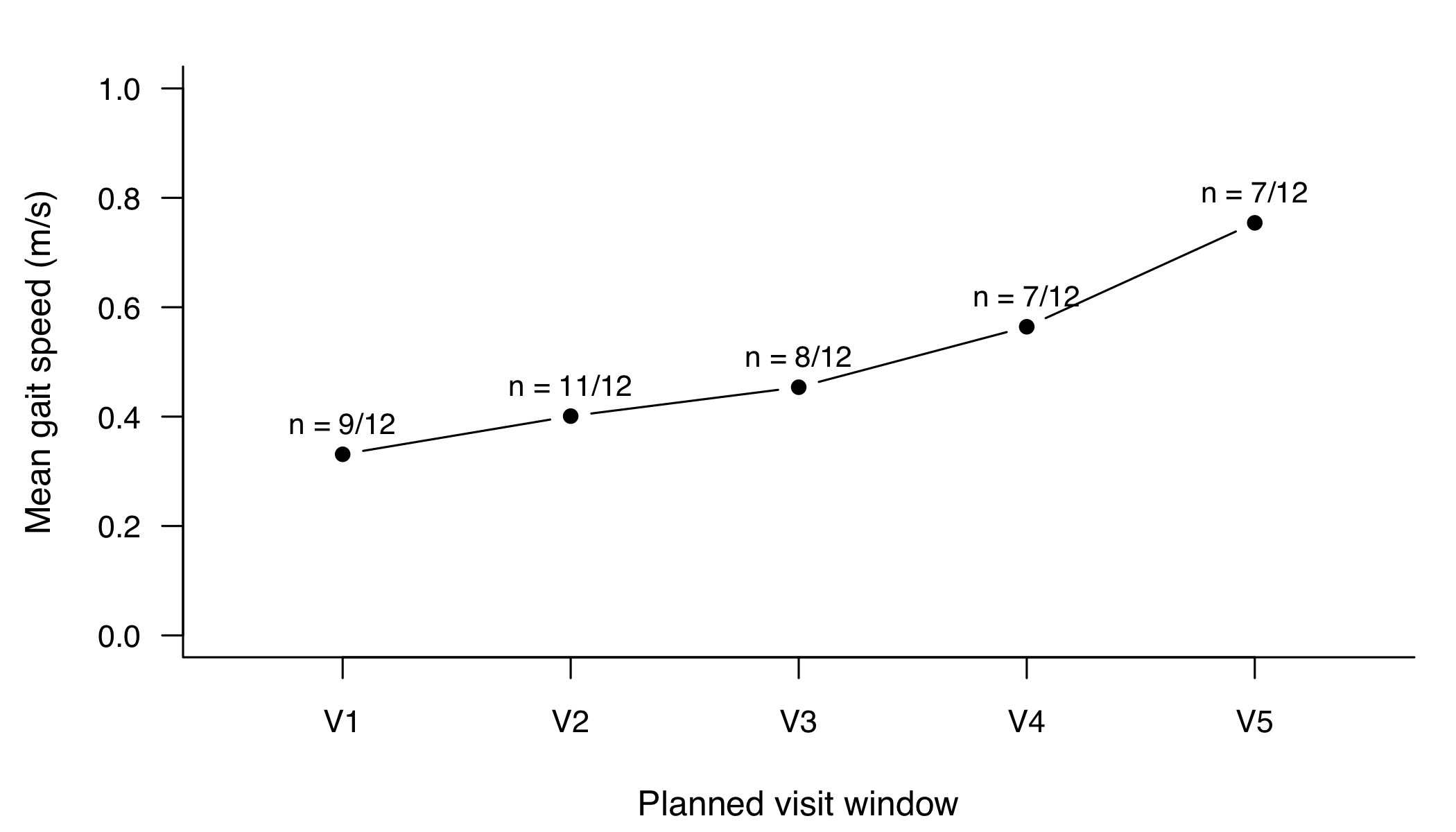
Base R line chart with five points for visit windows V1 to V5, rising from about 0.33 to 0.75 metres per second. Above the points the labels read n = 9/12, 11/12, 8/12, 7/12 and 7/12.
Figure 4.1: Mean gait speed (m/s) of the patients measured in each planned visit window (V1 days 1–3 to V5 days 80–100 after surgery), with the observed denominator above each point. Base R graphic. n = 12 patients; synthetic.
TipWhat you should see

Five points joined by lines, rising from left to right; the vertical axis runs from 0 to 1 m/s. The labels above the points read n = 9/12, n = 11/12, n = 8/12, n = 7/12 and n = 7/12. The fourth point, V4, lies just above 0.55 m/s: this is the target value of the project.

4.3.4 Step 4: long and wide

The table has one row per planned visit: the long format. Many spreadsheets use the wide format instead, with one row per patient and one column per visit. Base R’s reshape() converts between the two.

wide <- reshape(visits_b03[, c("pid", "window", "gait_ms")],
                idvar = "pid", timevar = "window", direction = "wide")
head(wide, 4)
#>    pid gait_ms.V1 gait_ms.V2 gait_ms.V3 gait_ms.V4 gait_ms.V5
#> 1  P01       0.31       0.42       0.55       0.63       0.78
#> 6  P02       0.28       0.35       0.47       0.58       0.70
#> 11 P03         NA       0.31       0.38         NA         NA
#> 16 P04       0.40       0.52         NA         NA       0.85
long_again <- reshape(wide, direction = "long")
stopifnot(dim(wide) == c(12, 6), nrow(long_again) == 60,
          sum(!is.na(wide[, -1])) == 42)      # still 42 measured values

The wide table looks tidier on screen but has lost two things: the actual day of each visit and the reason for each missing value. In the wide table, NA for patient P04 in V3 (at home) and NA for P05 in V3 (died) look identical. Wickham’s definition of tidy data — each variable a column, each observation a row, each type of observational unit a table — is the reason why the project keeps the long format and a separate patient table (Wickham 2014).

4.3.5 Step 5: start instructions and data schema

The README is the first file a colleague opens. It needs only four parts.

# hip-gait-project (synthetic teaching data)

## Start
1. Install R (version used: see output/session-info.txt) and Quarto.
2. Open a terminal in this folder and run:   Rscript run.R
3. Expected: "Done. Target value V4: 0.56 m/s (n = 7 of 12)". Any other result stops with an error.

## Data schema (data/raw/, read-only)
patients.csv   one row per patient     pid, age (years), sex, fracture, end_day (days since surgery), end_reason
visit_log.csv  one row per planned visit  pid, window (V1-V5), day (days since surgery), status
stopwatch.csv  one row per ward/outpatient test  pid, day, time_4m_s (seconds for 4 metres)
sensormat.csv  one row per rehabilitation test   pid, day, speed_cm_s (centimetres per second)
Key: pid (patients) = pid (all other files); pid + day identifies a test.

## Target value
Visit window V4: 7 of 12 patients measured, mean gait speed 0.564 m/s (rounded 0.56).

## Rights and data status
Synthetic data, CC BY 4.0. Code under MIT licence. See ARTEFACTS.csv.

The schema states the unit of every measurement column, and the units differ: seconds for 4 metres on the ward, centimetres per second on the sensor mat. The former manual division by 100 lived exactly here.

4.3.6 Step 6: the scripts

Each script defines one or two functions: named recipes that take an input and return an output. The first one is the planned-visit table of Chapter 3, copied unchanged; Step 7 checks that it really is unchanged.

# R/00_visits.R -- planned-visit table of chapter B03 (synthetic); one row = one planned visit
build_visits <- function() {
  windows <- c("V1", "V2", "V3", "V4", "V5")
  visit_rows <- function(pid, day, gait_ms, status) {
    data.frame(pid = pid, window = windows, day = day, gait_ms = gait_ms, status = status)
  }
  m <- "measured"
  visits <- rbind(
    visit_rows("P01", c(2, 6, 15, 27, 91), c(.31, .42, .55, .63, .78), rep(m, 5)),
    visit_rows("P02", c(1, 5, 13, 29, 88), c(.28, .35, .47, .58, .70), rep(m, 5)),
    visit_rows("P03", c(2, 6, 14, NA, NA), c(NA, .31, .38, NA, NA),
               c("unable", m, m, "transferred", "transferred")),
    visit_rows("P04", c(3, 8, NA, NA, 90), c(.40, .52, NA, NA, .85),
               c(m, m, "at home", "at home", m)),
    visit_rows("P05", c(1, 4, NA, NA, NA), c(NA, NA, NA, NA, NA),
               c("unable", "unable", "died", "died", "died")),
    visit_rows("P06", c(2, 7, 16, 30, NA), c(.33, .41, .50, .57, NA),
               c(m, m, m, m, "visit missed")),
    visit_rows("P07", c(2, 6, 12, 26, 93), c(.36, .47, .58, .66, .81), rep(m, 5)),
    visit_rows("P08", c(3, 8, 17, 31, NA), c(NA, .30, .29, NA, NA),
               c("unable", m, m, "unable", "transferred")),
    visit_rows("P09", c(2, 5, NA, NA, 90), c(.38, .49, NA, NA, .88),
               c(m, m, "at home", "at home", m)),
    visit_rows("P10", c(2, 9, 18, 28, 90), c(.27, .33, .41, .46, .52), rep(m, 5)),
    visit_rows("P11", c(1, 6, 15, 24, NA), c(.30, .37, .45, .44, NA), c(m, m, m, m, "died")),
    visit_rows("P12", c(3, 7, 14, 28, 89), c(.35, .44, NA, .61, .74),
               c(m, m, "device fault", m, m))
  )
  visits$method <- ifelse(visits$window %in% c("V3", "V4"), "sensor mat", "stopwatch")
  visits$method[is.na(visits$day)] <- NA
  visits
}
The second script turns this table into the files the devices and the clinic would deliver: a patient list, a visit log, a stopwatch export in seconds and a sensor-mat export in centimetres per second, including one duplicated row and one mistyped identifier, as in the case.

# R/01_simulate_raw.R -- raw exports (synthetic). In a real project: delivered files, read-only.
simulate_raw <- function() {
  patients <- data.frame(
    pid = sprintf("P%02d", 1:12),
    age = c(84, 79, 91, 76, 93, 82, 80, 88, 74, 86, 90, 78),
    sex = c("f", "f", "f", "m", "f", "f", "m", "f", "f", "m", "f", "f"),
    fracture = c("neck", "pertroch", "pertroch", "neck", "pertroch", "neck",
                 "neck", "pertroch", "neck", "pertroch", "neck", "neck"),
    end_day = c(91, 88, 20, 90, 11, 90, 93, 33, 90, 90, 52, 89),
    end_reason = c("follow-up complete", "follow-up complete", "transferred to nursing home",
                   "follow-up complete", "died", "day-90 visit missed", "follow-up complete",
                   "transferred to acute hospital", "follow-up complete", "follow-up complete",
                   "died", "follow-up complete"))
  visits <- build_visits()
  m <- visits[visits$status == "measured", ]
  ward <- m[m$method == "stopwatch", ]
  stopwatch <- data.frame(pid = ward$pid, day = ward$day,
                          time_4m_s = round(4 / ward$gait_ms, 2))        # seconds for 4 metres
  rehab <- m[m$method == "sensor mat", ]
  sensormat <- data.frame(pid = rehab$pid, day = rehab$day,
                          speed_cm_s = round(100 * rehab$gait_ms))       # centimetres per second
  sensormat <- rbind(sensormat, sensormat[sensormat$pid == "P02" & sensormat$day == 13, ])  # duplicate
  sensormat$pid[sensormat$pid == "P07" & sensormat$day == 12] <- "P7"                        # typing error
  list(patients = patients, visit_log = visits[, c("pid", "window", "day", "status")],
       stopwatch = stopwatch, sensormat = sensormat)
}

The third script replaces the hidden spreadsheet step. Every change is written down, and the function stops if the result is implausible or if a value cannot be linked to exactly one planned visit.

# R/02_clean.R -- documented cleaning instead of manual edits
id_corrections <- c(P7 = "P07")    # known typing error at the sensor mat, confirmed against the visit log

clean_visits <- function(raw) {
  sw <- raw$stopwatch
  sw$gait_ms <- round(4 / sw$time_4m_s, 2)            # 4 metres / seconds = metres per second
  sm <- raw$sensormat
  n_dup <- sum(duplicated(sm))
  sm <- sm[!duplicated(sm), ]                          # remove exact duplicate exports
  fix <- sm$pid %in% names(id_corrections)
  sm$pid[fix] <- id_corrections[sm$pid[fix]]           # correct known identifier errors
  sm$gait_ms <- sm$speed_cm_s / 100                    # centimetres per second -> metres per second
  values <- rbind(sw[c("pid", "day", "gait_ms")], sm[c("pid", "day", "gait_ms")])
  v <- raw$visit_log
  measured <- v$status == "measured"
  key_visit <- paste(v$pid, v$day)
  key_value <- paste(values$pid, values$day)
  stopifnot(!anyDuplicated(key_value),                 # one value per patient and day
            all(key_value %in% key_visit[measured]),   # every value belongs to a measured visit
            all(key_visit[measured] %in% key_value))   # every measured visit has a value
  v$gait_ms <- ifelse(measured, values$gait_ms[match(key_visit, key_value)], NA)
  stopifnot(all(v$gait_ms[measured] > 0.05 & v$gait_ms[measured] < 2.5))   # plausible range in m/s
  v$method <- ifelse(v$window %in% c("V3", "V4"), "sensor mat", "stopwatch")
  v$method[is.na(v$day)] <- NA
  v <- v[, c("pid", "window", "day", "gait_ms", "status", "method")]
  attr(v, "cleaning_log") <- c(duplicates_removed = n_dup, ids_corrected = sum(fix))
  v
}

The fourth script counts patients, measurements and linked records on two independent paths and stops if they disagree. The fifth script is the pair of figure functions from Step 3.

# R/03_check.R -- counts on two independent paths
check_counts <- function(visits, patients) {
  a <- c(patients     = length(unique(visits$pid)),                     # path A: visit table
         measurements = sum(visits$status == "measured"),
         linked       = sum(visits$pid[!is.na(visits$gait_ms)] %in% patients$pid))
  per_patient <- tapply(!is.na(visits$gait_ms), visits$pid, sum)       # path B: other objects
  b <- c(patients     = nrow(patients),
         measurements = sum(per_patient),
         linked       = nrow(merge(visits[!is.na(visits$gait_ms), ], patients, by = "pid")))
  stopifnot(identical(a, b), b[["patients"]] == 12, b[["measurements"]] == 42, b[["linked"]] == 42)
  b
}

4.3.7 Step 7: the one command, run inside this chapter

run.R calls the scripts in order and writes the files. Because a book chapter must not write project folders, the same sequence runs here in memory; the listing shows the file version.

# run.R -- one command, run from the project folder:  Rscript run.R
for (f in sort(list.files("R", pattern = "[.]R$", full.names = TRUE))) source(f)
dir.create(file.path("data", "raw"), recursive = TRUE, showWarnings = FALSE)
dir.create(file.path("data", "derived"), showWarnings = FALSE)
dir.create("output", showWarnings = FALSE)

raw <- simulate_raw()
for (nm in names(raw)) write.csv(raw[[nm]], file.path("data", "raw", paste0(nm, ".csv")), row.names = FALSE)
raw_in <- lapply(setNames(names(raw), names(raw)), function(nm)
  read.csv(file.path("data", "raw", paste0(nm, ".csv")), stringsAsFactors = FALSE))

visits <- clean_visits(raw_in)
write.csv(visits, file.path("data", "derived", "visits.csv"), row.names = FALSE)
counts <- check_counts(visits, raw_in$patients)
s <- summarise_windows(visits)
stopifnot(s$n[s$window == "V4"] == 7, abs(s$mean_ms[s$window == "V4"] - 0.564) < 0.001)   # target value

png(file.path("output", "figure-windows.png"), width = 1400, height = 900, res = 200)
draw_windows(s)
invisible(dev.off())
writeLines(capture.output(sessionInfo()), file.path("output", "session-info.txt"))
stopifnot(system2("quarto", c("render", file.path("report", "report.qmd"))) == 0)
cat("Done. Target value V4:", round(s$mean_ms[s$window == "V4"], 2), "m/s (n = 7 of 12)\n")

In memory, the CSV round trip is simulated with a text connection, so that the cleaning step sees exactly what it would read from disk.

as_csv_text <- function(df) capture.output(write.csv(df, row.names = FALSE))
from_csv_text <- function(lines) read.csv(text = lines, stringsAsFactors = FALSE)

raw <- simulate_raw()
raw_in <- lapply(raw, function(df) from_csv_text(as_csv_text(df)))
c(device_rows = nrow(raw_in$stopwatch) + nrow(raw_in$sensormat),
  unknown_ids = length(setdiff(c(raw_in$stopwatch$pid, raw_in$sensormat$pid), raw_in$patients$pid)))
#> device_rows unknown_ids 
#>          43           1
setdiff(raw_in$sensormat$pid, raw_in$patients$pid)    # which identifier cannot be linked
#> [1] "P7"
visits_new <- clean_visits(raw_in)
attr(visits_new, "cleaning_log")
#> duplicates_removed      ids_corrected 
#>                  1                  1
counts <- check_counts(visits_new, raw_in$patients)
counts
#>     patients measurements       linked 
#>           12           42           42
s <- summarise_windows(visits_new)
v4 <- s[s$window == "V4", ]
stopifnot(v4$n == 7, v4$of == 12, abs(v4$mean_ms - 0.564) < 0.001)    # target value

The raw exports contain 43 device rows, one of them with an identifier (P7) that does not exist in the patient list. After cleaning, the log reports one duplicate removed and one identifier corrected; the counts agree on both paths (12 patients, 42 measurements, 42 linked records), and the target value holds: in V4, 7 of 12 patients, mean 0.56 m/s.

The last check compares the result with the file that Chapter 3 wrote, cell by cell and as a cryptographic checksum (SHA-256, computed with the digest package). If a single character differed, the checksums would differ.

library(digest)
new_csv <- as_csv_text(visits_new)
b03_csv <- readLines(path_b03)
checksums <- c(rebuilt = digest(paste(new_csv, collapse = "\n"), algo = "sha256", serialize = FALSE),
               b03_file = digest(paste(b03_csv, collapse = "\n"), algo = "sha256", serialize = FALSE))
substr(checksums, 1, 16)                                   # first 16 of 64 hexadecimal characters
#>            rebuilt           b03_file 
#> "1b6e35d066ddaa31" "1b6e35d066ddaa31"
stopifnot(identical(from_csv_text(new_csv), visits_b03),   # same table, cell by cell
          checksums[["rebuilt"]] == checksums[["b03_file"]])

The table rebuilt from raw exports is identical to the one in Chapter 3. The number in the grant report can now be regenerated by anyone with the project folder.

4.3.8 Step 8: software version and report

sessionInfo() lists the R version, the operating system and the attached packages. Its output belongs at the end of every report.

print(sessionInfo(), locale = FALSE)
#> R version 4.6.1 (2026-06-24)
#> Platform: aarch64-apple-darwin27.0.0
#> Running under: macOS Golden Gate 27.0.1
#> 
#> Matrix products: default
#> BLAS:   /opt/homebrew/Cellar/openblas/0.3.34/lib/libopenblasp-r0.3.34.dylib 
#> LAPACK: /opt/homebrew/Cellar/r/4.6.1_1/lib/R/lib/libRlapack.dylib;  LAPACK version 3.12.1
#> 
#> attached base packages:
#> [1] stats     graphics  grDevices utils     datasets  methods   base     
#> 
#> other attached packages:
#> [1] digest_0.6.39
#> 
#> loaded via a namespace (and not attached):
#>  [1] htmlwidgets_1.6.4 compiler_4.6.1    fastmap_1.2.0     cli_3.6.6        
#>  [5] tools_4.6.1       htmltools_0.5.9   otel_0.2.0        yaml_2.3.12      
#>  [9] rmarkdown_2.32    knitr_1.52        jsonlite_2.0.0    xfun_0.62        
#> [13] rlang_1.3.0       evaluate_1.0.5

The Quarto report computes every number it mentions. The r inside back-ticks in the text below is evaluated when the report is rendered.

---
title: "Gait speed after hip fracture surgery (synthetic teaching data)"
format: html
---

```{r}
#| include: false
source("../R/04_figure.R")
visits <- read.csv("../data/derived/visits.csv", stringsAsFactors = FALSE)
s <- summarise_windows(visits)
v4 <- s[s$window == "V4", ]
```

In visit window V4 (days 21–35), `r v4$n` of `r v4$of` patients were measured.
Their mean gait speed was `r sprintf("%.2f", v4$mean_ms)` m/s (@fig-windows).

```{r}
#| label: fig-windows
#| fig-cap: "Mean gait speed per visit window; n = patients measured of 12 (synthetic)."
#| fig-alt: "Line chart of mean gait speed in five visit windows with the number of measured patients above each point."
draw_windows(s)
```

```{r}
sessionInfo()
```

4.3.9 Step 9: version control with Git

Git is run in a terminal, not in R. The commands below put the project under version control; the file .gitignore lists what Git should never record. Derived files are excluded because run.R regenerates them. In a project with real patient data, the raw data folder belongs in .gitignore too: a file that was committed once remains in the history even after it is deleted.

git init                                   # start recording in this folder
git add README.md run.R R/ report/report.qmd .gitignore
git commit -m "Rebuild gait figure from raw exports; target value V4 = 0.56 m/s"
git log --oneline                          # list of recorded versions
# .gitignore
data/derived/
output/
report/report.html
report/report_files/

4.3.10 Step 10: the artefact register

The passport of Table 4.1 can itself be produced by code, with a checksum for each data file so that a later reader can verify that the file in hand is the file described.

sha <- function(lines) substr(digest(paste(lines, collapse = "\n"), algo = "sha256", serialize = FALSE), 1, 12)
artefacts <- data.frame(
  artefact    = c(paste0("data/raw/", names(raw_in), ".csv"), "data/derived/visits.csv"),
  produced_by = c(rep("R/01_simulate_raw.R", 4), "R/02_clean.R"),
  rights      = "CC BY 4.0",
  data_status = "synthetic",
  rows        = c(sapply(raw_in, nrow), nrow(visits_new)),
  sha256_start = c(sapply(raw, function(df) sha(as_csv_text(df))), sha(new_csv))
)
artefacts
#>                          artefact         produced_by    rights data_status
#> patients    data/raw/patients.csv R/01_simulate_raw.R CC BY 4.0   synthetic
#> visit_log  data/raw/visit_log.csv R/01_simulate_raw.R CC BY 4.0   synthetic
#> stopwatch  data/raw/stopwatch.csv R/01_simulate_raw.R CC BY 4.0   synthetic
#> sensormat  data/raw/sensormat.csv R/01_simulate_raw.R CC BY 4.0   synthetic
#>           data/derived/visits.csv        R/02_clean.R CC BY 4.0   synthetic
#>           rows sha256_start
#> patients    12 1b4cbc97ca03
#> visit_log   60 ba8abf3cbfe3
#> stopwatch   27 1a5c3dbdeda2
#> sensormat   16 42ee1164c4e8
#>             60 1b6e35d066dd
stopifnot(artefacts$rows == c(12, 60, 27, 16, 60))

The register shows 12 patients, 60 planned visits, 27 stopwatch rows and 16 sensor-mat rows (15 tests plus the duplicate). Saved as ARTEFACTS.csv next to the README, it answers the three questions of the passport for every data file.

4.4 Counter-check

A firmware update of the sensor mat changes its export from centimetres per second to metres per second, without notice. The project is run again unchanged. Predict first: does the run finish with a wrong target value, finish with the right one, or stop — and at which line?

raw_updated <- raw_in
raw_updated$sensormat$speed_cm_s <- raw_updated$sensormat$speed_cm_s / 100   # now really m/s
outcome <- tryCatch({
  clean_visits(raw_updated)
  "run finished"
}, error = function(e) conditionMessage(e))
outcome
#> [1] "all(v$gait_ms[measured] > 0.05 & v$gait_ms[measured] < 2.5) is not TRUE"
stopifnot(outcome != "run finished")

The run stops inside clean_visits() at the plausibility check: after the now superfluous division by 100, rehabilitation values of about 0.005 m/s fall outside the range of 0.05 to 2.5 m/s. Without that line, the target value check would have caught the error one step later, because the V4 mean would have collapsed. In the spreadsheet version of the project, the same firmware update would have produced a plausible-looking figure with nonsense in two of its five points. A check that can fail is what turns a script into evidence.

4.5 Consequences for patients and operations

Patients. An unreproducible number in a grant report or a publication can steer resources and clinical practice. Patients are not harmed by a missing script directly, but by a decision based on a number nobody can check. The target value and the two-path count make a silent error visible before it travels.

Operations. A department can adopt three simple rules: raw exports are stored read-only; every reported number comes from a script with a target value; and every exported file has a passport like Table 4.1. Device changes such as the firmware update need a change log that the analysis team can see.

Data protection and information security. Version control, cloud storage and code-sharing platforms are copies. For real patient data, the rule is: code and documentation may be shared under the conditions agreed, data are not committed. A raw file that once entered a Git history remains there until the history is rewritten, which is a security incident to be handled, not a clean-up task (Chapter 24). Pseudonymised identifiers such as P01 remain personal data under the GDPR (European Parliament and Council of the European Union 2016); the key that links them to names is kept apart from the project (Chapter 23). Which platform an institution permits for which data class is a local decision (open, to be clarified with the data protection officer and IT security).

Rights. In this book, text and figures are licensed under CC BY 4.0 and code under the MIT licence. In a research project the rights column must name the actual terms: data use agreements, ethics approval, and third-party material such as device manuals or published figures.

4.6 Look up and transfer

  • Reviewer question: Can the number in the main figure be regenerated from the raw data with the published code and a single command, and is there a stated target value that the code checks?

  • Self-test: A colleague sends you analysis.R. It starts with setwd("C:/Users/maria/Documents/thesis"), loads data_final_clean.csv and draws the figure. There is no other file. List three things you need before you can say whether the figure is reproducible.

    1. The raw data and the code that produced data_final_clean.csv from them; “final clean” suggests hidden steps.
    2. A project folder with relative paths instead of setwd() to a personal directory, so that it runs on another computer. (3) A target value (the number the figure should show) and the software versions (sessionInfo()); with random elements also the seed. Useful in addition: a data dictionary with units and the Git history.
  • Annotated sources:

    • Peng (2011) — reproducibility as the minimum standard for computational claims.
    • Sandve et al. (2013) — ten rules, five of which structure the project in this chapter.
    • Wilson et al. (2017) — practical project organisation for researchers without programming training.
    • Ziemann et al. (2016) — a published example of silent spreadsheet conversions in the literature.
    • Wickham (2014) — the definition of tidy (long) data used for the visit table.
    • Bryan (2018) — Git for statistical work, written for beginners.
    • Quarto (n.d.) and R Core Team (2026) — the publishing system and the R software used.

4.7 Further reading