library(ggplot2)
library(dagitty)
library(lme4)
library(splines)Lab W5 · Collider, mixed model and clusters
Teaching units 17–19: selection on ICU admission as a collider, biomarker trajectories with informative late dropout in a mixed model, and two elective stations on clusters and flexible time functions.
The setting is a fictitious cohort of people with traumatic spinal cord injury. Every number on this page is synthetic or a teaching assumption: the biomarker levels, the effect sizes and the reasons why samples are missing were chosen to make one methodological point at a time. None of them describes real patients, a real laboratory or a real intensive care unit.
Each part follows the same five steps: state the decision, look at the data, name the assumption, compute in R and write one sentence for the person who has to act. Everyone works through Parts A and B. In Part C each group chooses one of two stations and presents its finding to the other group.
If R is new to you, read the code and the printed output first and answer the questions on paper; the printed results are complete. If you are fluent in R, change the parameters named in the counter-checks and rerun the script.
Part A · Selecting on ICU admission (unit 17)
Decision. A research group holds a registry of patients admitted to intensive care after spinal cord injury. They see that patients with a higher serum biomarker on admission have lower motor scores at six months, and they ask whether a drug that lowers the biomarker would improve recovery. Before anyone plans a trial, the group has to say which question they are asking. A prognostic question asks whether the biomarker helps to predict the outcome among ICU patients. A causal question asks what would happen to the outcome if the biomarker were changed by an intervention. The second question needs a causal argument, not only an association.
Assumption. The causal structure below is an assumption written down before looking at the data. Injury severity and a low biomarker both make ICU admission more likely; only severity affects the motor score. By construction there is no arrow from the biomarker to the outcome.
# Part A (unit 17): assumed causal structure. Severity and the biomarker both influence ICU admission;
# only severity influences the outcome. The biomarker has NO effect on the outcome by construction.
dag <- dagitty("dag {
  severity -> icu
  biomarker -> icu
  severity -> outcome
}")
coordinates(dag) <- list(x = c(severity = 0, biomarker = 2, icu = 1, outcome = 0),
                         y = c(severity = 0, biomarker = 0, icu = 1, outcome = 2))
# Which variables must be adjusted for to estimate the effect of the biomarker on the outcome?
adjustmentSets(dag, exposure = "biomarker", outcome = "outcome")
#> {}# Are biomarker and outcome independent ...
c(unconditional = dseparated(dag, "biomarker", "outcome", list()),
given_icu = dseparated(dag, "biomarker", "outcome", "icu"),
given_icu_and_severity = dseparated(dag, "biomarker", "outcome", c("icu", "severity")))#> unconditional given_icu given_icu_and_severity
#> TRUE FALSE TRUEstopifnot(dseparated(dag, "biomarker", "outcome", list()), # independent in everyone
!dseparated(dag, "biomarker", "outcome", "icu"), # selecting on ICU opens a path
dseparated(dag, "biomarker", "outcome", c("icu", "severity"))) # adjusting for severity closes itnodes <- data.frame(name = c("severity", "biomarker", "icu", "outcome"),
label = c("Injury severity", "Serum biomarker", "ICU admission\n(selection)", "Motor score\nat 6 months"),
x = c(0, 2, 1, 0), y = c(2, 2, 1, 0))
edges <- data.frame(from = c("severity", "biomarker", "severity"), to = c("icu", "icu", "outcome"))
edges <- cbind(edges,
setNames(nodes[match(edges$from, nodes$name), c("x", "y")], c("x", "y")),
setNames(nodes[match(edges$to, nodes$name), c("x", "y")], c("xend", "yend")))
shorten <- function(a, b, by = 0.22) a + (b - a) * (1 - by / sqrt(sum((b - a)^2))) # stop arrows before labels
for (i in seq_len(nrow(edges))) {
end <- shorten(c(edges$x[i], edges$y[i]), c(edges$xend[i], edges$yend[i]))
start <- shorten(c(edges$xend[i], edges$yend[i]), c(edges$x[i], edges$y[i]))
edges[i, c("x", "y", "xend", "yend")] <- c(start, end)
}
p_dag <- ggplot() +
geom_segment(data = edges, aes(x = x, y = y, xend = xend, yend = yend),
arrow = arrow(length = unit(0.25, "cm"), type = "closed"), colour = cdsr_colours[["grey"]]) +
geom_label(data = nodes, aes(x = x, y = y, label = label,
fill = ifelse(name == "icu", "selection", "variable")),
size = 3.6, linewidth = 0.3, show.legend = FALSE) +
scale_fill_manual(values = c(selection = "#F6D9A8", variable = "white")) +
annotate("text", x = 1.05, y = 0.25, size = 3.3, colour = cdsr_colours[["red"]],
label = "No arrow from biomarker to outcome:\nany association is not causal") +
scale_x_continuous(limits = c(-0.5, 2.5)) + scale_y_continuous(limits = c(-0.3, 2.3)) +
labs(caption = "Assumed causal structure for the teaching case (assumption, not a finding).") +
theme_void(base_size = 12) +
theme(plot.caption = element_text(hjust = 0, colour = "#4D4D4D", size = rel(0.8)))
show_figure(p_dag, "w5-dag.png", width = 7, height = 4.5)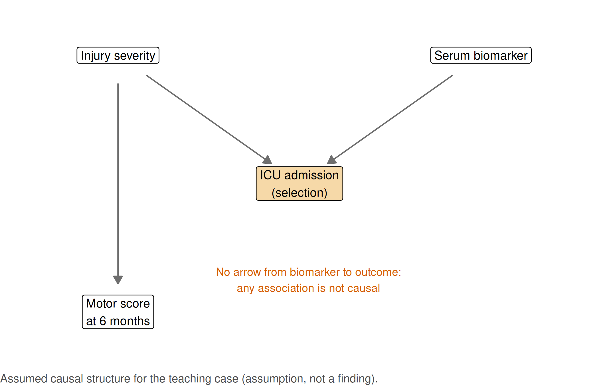
adjustmentSets() returns the empty set: in the whole population nothing needs to be adjusted for, because there is no open path from the biomarker to the outcome. dseparated() shows what changes when we condition on ICU admission. Restricting the analysis to ICU patients is exactly such a conditioning step.
Look at the data and compute. We simulate 5,000 patients according to the graph and compare the association between biomarker and motor score in everyone, in ICU patients only, and in ICU patients with adjustment for severity.
# Simulate 5,000 patients according to the DAG
set.seed(20260517)
n <- 5000
cohort <- data.frame(id = sprintf("SCI%04d", seq_len(n)))
cohort$severity  <- rnorm(n)                                    # standardised severity score
cohort$biomarker <- round(rnorm(n, 80, 15), 1)                  # serum biomarker, µg/L (synthetic)
# Low biomarker values and high severity both prompt ICU admission
p_icu <- plogis(-1.2 + 1.6 * cohort$severity - 0.08 * (cohort$biomarker - 80))
cohort$icu <- rbinom(n, 1, p_icu)
# Outcome depends on severity only (points on a synthetic 0-100 motor scale)
cohort$motor_score <- round(pmin(100, pmax(0, 55 - 9 * cohort$severity + rnorm(n, 0, 8))), 1)

# Association of the biomarker with the outcome, per 10 µg/L
per10 <- function(fit) 10 * unname(coef(fit)["biomarker"])
icu_only <- cohort[cohort$icu == 1, ]
collider_table <- data.frame(
  analysis = c("All patients", "ICU patients only", "ICU patients only, adjusted for severity"),
  patients = c(nrow(cohort), nrow(icu_only), nrow(icu_only)),
  slope_per_10 = c(per10(lm(motor_score ~ biomarker, data = cohort)),
                   per10(lm(motor_score ~ biomarker, data = icu_only)),
                   per10(lm(motor_score ~ biomarker + severity, data = icu_only)))
)
print(collider_table, digits = 3)
#> analysis patients slope_per_10
#> 1 All patients 5000 0.0318
#> 2 ICU patients only 1588 -1.0459
#> 3 ICU patients only, adjusted for severity 1588 -0.0015stopifnot(
abs(collider_table$slope_per_10[1]) < 0.3, # no association in the whole population
collider_table$slope_per_10[2] < -0.8, # spurious negative association after selection on ICU
abs(collider_table$slope_per_10[3]) < 0.3 # adjusting for severity closes the opened path
)plot_df <- rbind(data.frame(panel = "All patients", cohort[, c("biomarker", "motor_score")]),
data.frame(panel = "ICU patients only", icu_only[, c("biomarker", "motor_score")]))
plot_df$panel <- factor(plot_df$panel, levels = c("All patients", "ICU patients only"))
p_collider <- ggplot(plot_df, aes(biomarker, motor_score)) +
geom_point(alpha = 0.15, size = 0.8, colour = cdsr_colours[["grey"]]) +
geom_smooth(method = "lm", formula = y ~ x, se = TRUE, colour = cdsr_colours[["blue"]]) +
facet_wrap(~ panel) +
labs(x = "Serum biomarker (µg/L)", y = "Motor score at 6 months (points)",
caption = sprintf("Synthetic cohort; n = %s patients in total, %s admitted to ICU. Line = linear fit with 95%% band.",
cdsr_number(nrow(cohort)), cdsr_number(nrow(icu_only)))) +
theme_cdsr()
show_figure(p_collider, "w5-collider.png")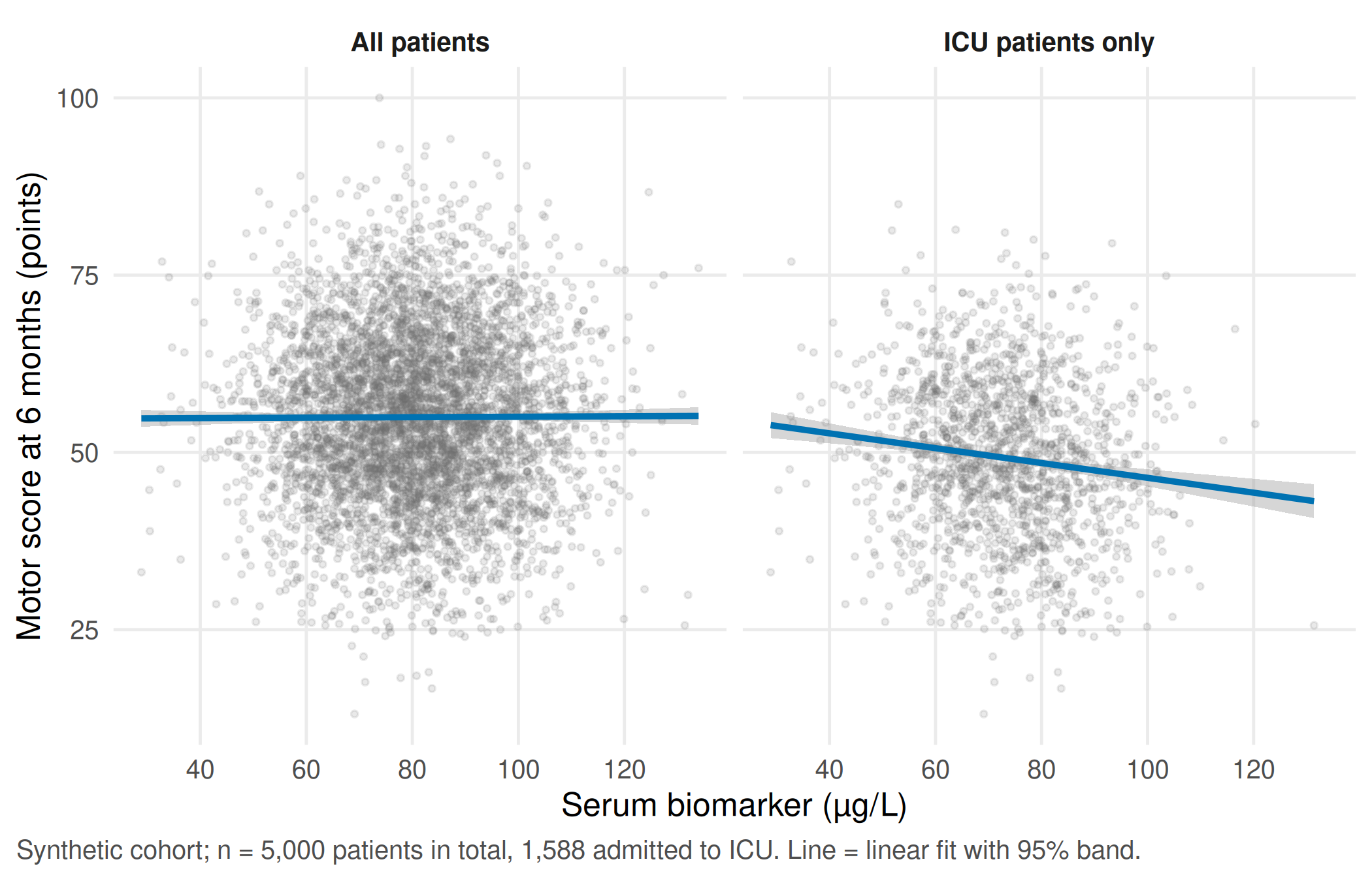
knitr::kable(collider_table, digits = 2,
col.names = c("Analysis", "Patients", "Change per 10 µg/L (points)"))| Analysis | Patients | Change per 10 µg/L (points) |
|---|---|---|
| All patients | 5000 | 0.03 |
| ICU patients only | 1588 | -1.05 |
| ICU patients only, adjusted for severity | 1588 | 0.00 |
Report. In all 5,000 patients the biomarker is unrelated to the motor score (+0.03 points per 10 µg/L). Among the 1,588 ICU patients the same data show -1.05 points per 10 µg/L, although the biomarker has no effect at all. Among ICU patients a high biomarker “signals” that admission must have been driven by severe injury, and severe injury lowers the motor score. Within the registry the association may still help to predict outcomes; it is no reason to expect benefit from lowering the biomarker.
TipCounter-check: predict first
Suppose ICU admission depended on severity only, not on the biomarker. Does the association among ICU patients stay negative, vanish or turn positive? Write down your guess, then run the chunk.
# Counter-check: same patients, but ICU admission now depends on severity only
set.seed(20260520)
icu_severity_only <- rbinom(n, 1, plogis(-1.2 + 1.6 * cohort$severity))
slope_counter <- per10(lm(motor_score ~ biomarker, data = cohort[icu_severity_only == 1, ]))
slope_counter
#> [1] 0.03993876stopifnot(abs(slope_counter) < 0.3) # ICU is no longer a collider between biomarker and severityWith admission driven by severity alone, ICU admission is no longer a common effect of biomarker and severity, and the association among ICU patients is +0.04 points per 10 µg/L.
WarningCommon mistake
“We adjusted for everything we had.” Adjusting for, or selecting on, a common effect of the exposure and of a cause of the outcome (here ICU admission) can create an association where none existed. Decide on adjustment variables from the assumed causal structure, not from availability or p-values.
Part B · Trajectories with late dropout (unit 18)
Decision. Does the serum biomarker rise faster in the first four weeks after an incomplete lesion than after a complete lesion? The answer is to be reported as a difference in rise per week, with its uncertainty, the number of persons and a statement about missing samples.
Look at the data. Forty persons (20 per group) are sampled on days 1, 3, 7, 14 and 28. Draw the trajectories before fitting any model: each line is one person.
# Part B (unit 18): biomarker trajectories in 40 persons, measured on days 1, 3, 7, 14 and 28
set.seed(20260518)
days <- c(1, 3, 7, 14, 28)
persons <- data.frame(id = sprintf("P%02d", 1:40),
                      lesion = factor(rep(c("complete", "incomplete"), each = 20),
                                      levels = c("complete", "incomplete")))
persons$u0 <- rnorm(40, 0, 6)      # person-specific starting level, µg/L
persons$u1 <- rnorm(40, 0, 1.5)    # person-specific slope, µg/L per week
full <- merge(persons, data.frame(day = days))
full <- full[order(full$id, full$day), ]
full$week <- full$day / 7
mean_slope <- ifelse(full$lesion == "complete", 5, 8)            # initial rise, µg/L per week (assumption)
full$selenium <- round(60 + full$u0 + (mean_slope + full$u1) * full$week -
                         0.8 * full$week^2 + rnorm(nrow(full), 0, 3), 1)   # rise levels off (assumption)

# Informative dropout: the lower a person's (unobserved) day-28 value, the likelier the day-28 sample is missing
day28 <- full[full$day == 28, ]
p_missing <- plogis(-1.0 - 0.25 * (day28$selenium - median(day28$selenium)))
missing_ids <- day28$id[rbinom(nrow(day28), 1, p_missing) == 1]
full$observed <- !(full$day == 28 & full$id %in% missing_ids)
obs <- full[full$observed, c("id", "lesion", "day", "week", "selenium")]
c(persons = length(unique(obs$id)), observations = nrow(obs), missing_day28 = length(missing_ids))
#> persons observations missing_day28
#> 40 188 12table(lesion = persons$lesion, missing_day28 = persons$id %in% missing_ids)#> missing_day28
#> lesion FALSE TRUE
#> complete 11 9
#> incomplete 17 3stopifnot(length(unique(obs$id)) == 40, nrow(obs) == 200 - length(missing_ids),
length(missing_ids) >= 8)obs$dropped_out <- ifelse(obs$id %in% missing_ids, "day-28 sample missing", "complete series")
p_spaghetti <- ggplot(obs, aes(day, selenium, group = id, colour = dropped_out, linetype = dropped_out)) +
geom_line(alpha = 0.7) +
geom_point(size = 1) +
facet_wrap(~ lesion, labeller = labeller(lesion = c(complete = "Complete lesion", incomplete = "Incomplete lesion"))) +
scale_colour_manual(values = c("complete series" = cdsr_colours[["blue"]],
"day-28 sample missing" = cdsr_colours[["red"]])) +
scale_linetype_manual(values = c("complete series" = "solid", "day-28 sample missing" = "22")) +
scale_x_continuous(breaks = days) +
labs(x = "Day after injury", y = "Serum selenium (µg/L)", colour = NULL, linetype = NULL,
caption = sprintf("Synthetic data; n = 40 persons (20 per group), %d observations; %d persons without a day-28 sample.",
nrow(obs), length(missing_ids))) +
theme_cdsr()
show_figure(p_spaghetti, "w5-spaghetti.png")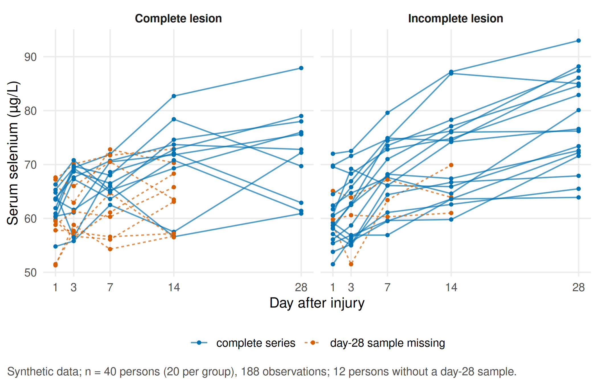
The unit of analysis is the person, not the observation: there are 188 observations but only 40 independent persons. No day-28 sample is available for 12 persons, most of them in the complete-lesion group.
Assumption. In this synthetic cohort the day-28 sample is more likely to be missing when the person’s day-28 value would have been low, for example because people who are doing poorly are transferred before the last sample. Missingness that depends on the unobserved value itself is called missing not at random (MNAR). With real data this cannot be checked from the observed values; it can only be explored with a sensitivity analysis.
Compute, step 1: a simple summary per person. Fit one straight line per person and compare the mean slopes of the two groups.
# Simple analysis: one least-squares slope per person (µg/L per week), then compare the groups
person_slopes <- do.call(rbind, lapply(split(obs, obs$id), function(d)
  data.frame(id = d$id[1], lesion = d$lesion[1], n_obs = nrow(d),
             slope = unname(coef(lm(selenium ~ week, data = d))["week"]))))
aggregate(slope ~ lesion, data = person_slopes, FUN = mean)
#> lesion slope
#> 1 complete 2.262952
#> 2 incomplete 4.171081summary_test <- t.test(slope ~ lesion, data = person_slopes)
summary_diff <- unname(diff(summary_test$estimate)) # incomplete minus complete
summary_test#>
#> Welch Two Sample t-test
#>
#> data: slope by lesion
#> t = -2.9679, df = 37.998, p-value = 0.005166
#> alternative hypothesis: true difference in means between group complete and group incomplete is not equal to 0
#> 95 percent confidence interval:
#> -3.2096586 -0.6065993
#> sample estimates:
#> mean in group complete mean in group incomplete
#> 2.262952 4.171081Compute, step 2: a linear mixed model. One model for all observations, with a random intercept and a random slope per person and an interaction between time and lesion type. The interaction is the difference in rise per week between the groups.
# Linear mixed model: random intercept and slope per person, time-by-group interaction
fit_mixed <- lmer(selenium ~ week * lesion + (1 + week | id), data = obs)
stopifnot(!isSingular(fit_mixed))
summary(fit_mixed)$coefficients
#> Estimate Std. Error t value
#> (Intercept) 62.211345 1.1271792 55.1920615
#> week 2.252081 0.4279248 5.2627973
#> lesionincomplete -1.095012 1.5875321 -0.6897574
#> week:lesionincomplete 2.050859 0.5720738 3.5849558interaction_est <- unname(fixef(fit_mixed)["week:lesionincomplete"])
interaction_ci <- unname(confint(fit_mixed, parm = "week:lesionincomplete", method = "Wald")[1, ])
c(estimate = interaction_est, lower = interaction_ci[1], upper = interaction_ci[2])#> estimate lower upper
#> 2.0508592 0.9296152 3.1721032stopifnot(interaction_ci[1] > 0) # steeper rise with incomplete lesions in this synthetic cohortCompute, step 3: what the dropout does to the day-28 mean. Because the data are synthetic, we also know the day-28 values that would have been measured without dropout. A real study never has this column.
# What does the late dropout do to the day-28 mean? Because the data are synthetic, the values that
# would have been measured without dropout are known and serve as the reference.
# A straight line would distort the day-28 mean, so this model estimates one mean per day and group,
# with the same random intercept and slope per person.
fit_days <- lmer(selenium ~ factor(day) * lesion + (1 + week | id), data = obs)
stopifnot(!isSingular(fit_days))
grid28 <- data.frame(day = 28, week = 4,
                     lesion = factor(c("complete", "incomplete"), levels = levels(obs$lesion)))
day28_table <- data.frame(
  lesion = grid28$lesion,
  without_dropout = as.vector(tapply(full$selenium[full$day == 28], full$lesion[full$day == 28], mean)),
  completers_only = as.vector(tapply(obs$selenium[obs$day == 28], obs$lesion[obs$day == 28], mean)),
  mixed_model     = unname(predict(fit_days, newdata = grid28, re.form = NA))
)
print(day28_table, digits = 3, row.names = FALSE)
#> lesion without_dropout completers_only mixed_model
#> complete 68.2 72.4 69.2
#> incomplete 76.4 78.1 77.1bias_completers <- with(day28_table, completers_only - without_dropout)
bias_mixed <- with(day28_table, mixed_model - without_dropout)
stopifnot(all(bias_completers > 0), # completers look better than everyone
all(abs(bias_mixed) < bias_completers)) # using all earlier measurements helpsknitr::kable(day28_table, digits = 1, row.names = FALSE,
col.names = c("Lesion", "Without dropout (reference)", "Completers only", "Mixed model, one mean per day"))| Lesion | Without dropout (reference) | Completers only | Mixed model, one mean per day |
|---|---|---|---|
| complete | 68.2 | 72.4 | 69.2 |
| incomplete | 76.4 | 78.1 | 77.1 |
Compute, step 4: sensitivity analysis. Fill the missing day-28 values with each person’s own model prediction minus δ, for δ = 0, 5 and 10 µg/L, and refit. δ = 0 corresponds to “missing at random given the earlier values”; larger δ means “those who were not sampled were doing worse than their earlier values suggest”.
# Sensitivity analysis (delta adjustment): missing day-28 values are filled with each person's own
# prediction (including their random effects) minus delta, i.e. "those without a day-28 sample did
# delta µg/L worse than their earlier values suggest".
missing_rows <- full[!full$observed, c("id", "lesion", "day", "week")]
pred_missing <- predict(fit_days, newdata = missing_rows)
sensitivity_table <- do.call(rbind, lapply(c(0, 5, 10), function(delta) {
  filled <- rbind(obs[, c("id", "lesion", "day", "week", "selenium")],
                  cbind(missing_rows, selenium = pred_missing - delta))
  refit <- lmer(selenium ~ week * lesion + (1 + week | id), data = filled)
  data.frame(delta = delta,
             mean_day28_complete   = mean(filled$selenium[filled$day == 28 & filled$lesion == "complete"]),
             mean_day28_incomplete = mean(filled$selenium[filled$day == 28 & filled$lesion == "incomplete"]),
             interaction = unname(fixef(refit)["week:lesionincomplete"]))
}))
print(sensitivity_table, digits = 3, row.names = FALSE)
#> delta mean_day28_complete mean_day28_incomplete interaction
#> 0 69.2 77.1 2.29
#> 5 66.9 76.3 2.67
#> 10 64.7 75.6 3.05stopifnot(all(diff(sensitivity_table$mean_day28_complete) < 0),
all(sensitivity_table$interaction > 0))Report. In 40 persons with 188 observations, serum selenium rose by 2.1 µg/L per week more after incomplete than after complete lesions (95% CI 0.9 to 3.2; linear mixed model with random intercept and slope). The simple per-person slopes give a similar difference (1.9 µg/L per week). No day-28 sample was available for 12 persons; completers alone overstate the day-28 mean of the complete-lesion group by 4.2 µg/L. If the missing values were 10 µg/L lower than predicted, the difference in rise would be 3.1 µg/L per week: the direction of the finding holds, its size depends on an assumption about the missing samples.
TipCounter-check: predict first
Before you look at the sensitivity table: as δ grows, will the estimated difference between the groups shrink or grow? Which group loses more when δ increases, and why?
WarningCommon mistake
Reporting the mean of the completers at day 28 as “the day-28 value”. Here the completers are the persons who were doing better, so the mean is too high, and it is too high by different amounts in the two groups.
Part C · Elective stations (unit 19)
Each group works on one station for about 30 minutes and then explains its result to the other group in five minutes: what was the alternative explanation, and which plot or number supports the conclusion?
Station 1 · Cluster, gradient or artefact
Decision. A team proposes three “inflammatory subtypes” of patients based on four admission markers and wants to use them to stratify a future trial. Are there three groups, or one continuous gradient cut into three pieces?
Look at the data. The synthetic markers of 300 patients are generated from a single continuous gradient (three markers) plus one unrelated marker on a large numerical scale. Compare the standard deviations of the raw markers.
# Part C, cluster station (unit 19): 300 patients lie on ONE continuous gradient (e.g. inflammatory
# activity) that drives three markers; a fourth marker is pure noise on a large numerical scale
set.seed(20260519)
m <- 300
gradient <- runif(m)
markers <- data.frame(
  marker_a = 10 + 30 * gradient + rnorm(m, 0, 3),      # mg/L
  marker_b = 200 - 80 * gradient + rnorm(m, 0, 10),    # U/L
  marker_c = 2 + 1.5 * gradient + rnorm(m, 0, 0.2),    # ratio
  marker_d = rnorm(m, 500, 120)                        # unrelated, large scale
)
round(sapply(markers, sd), 1)
#> marker_a marker_b marker_c marker_d
#> 9.3 26.1 0.5 117.3Assumption. k-means always returns the requested number of clusters, whether or not groups exist. Distances on raw values are dominated by the marker with the largest numerical spread.
# k-means with k = 3 on raw values and on standardised values
set.seed(1)
km_raw    <- kmeans(markers, centers = 3, nstart = 25)
set.seed(1)
km_scaled <- kmeans(scale(markers), centers = 3, nstart = 25)
ari_raw_scaled <- mclust::adjustedRandIndex(km_raw$cluster, km_scaled$cluster)
# Are the "clusters" just cuts of the gradient? Rank correlation of cluster (ordered by mean gradient) with the gradient
order_by_gradient <- function(cl) rank(tapply(gradient, cl, mean))[cl]
rho_scaled <- cor(order_by_gradient(km_scaled$cluster), gradient, method = "spearman")
rho_raw    <- cor(order_by_gradient(km_raw$cluster), gradient, method = "spearman")
c(adjusted_rand_raw_vs_scaled = ari_raw_scaled, rho_scaled = rho_scaled, rho_raw = rho_raw)
#> adjusted_rand_raw_vs_scaled rho_scaled
#> 0.04526047 0.89929098
#> rho_raw
#> 0.08297290# Bootstrap stability of the standardised solution: recluster resamples, compare on the resampled patients
set.seed(2)
z <- scale(markers)
boot_ari <- replicate(50, {
idx <- sample(m, replace = TRUE)
km_b <- kmeans(z[idx, ], centers = 3, nstart = 10)
mclust::adjustedRandIndex(km_b$cluster, km_scaled$cluster[idx])
})
summary(boot_ari)#> Min. 1st Qu. Median Mean 3rd Qu. Max.
#> 0.3707 0.5088 0.6589 0.6731 0.8119 0.9902# Mean silhouette width: values below about 0.5 do not indicate well-separated groups
sil <- cluster::silhouette(km_scaled$cluster, dist(z))
mean_silhouette <- mean(sil[, "sil_width"])
mean_silhouette#> [1] 0.2988153stopifnot(ari_raw_scaled < 0.2, # the two scalings give unrelated partitions
rho_raw < 0.3, # raw-scale clusters follow the large-scale noise marker
rho_scaled > 0.85, # standardised clusters are essentially slices of the gradient
median(boot_ari) > 0.5, # moderately reproducible, which still would not prove distinct groups
mean_silhouette < 0.4) # weak separationpca <- prcomp(z)
cl_df <- data.frame(pc1 = pca$x[, 1], gradient = gradient,
scaled = factor(order_by_gradient(km_scaled$cluster)),
raw = factor(order_by_gradient(km_raw$cluster)))
cl_long <- rbind(data.frame(scaling = "Standardised markers", cl_df[, c("pc1", "gradient")], cluster = cl_df$scaled),
data.frame(scaling = "Raw markers", cl_df[, c("pc1", "gradient")], cluster = cl_df$raw))
cl_long$scaling <- factor(cl_long$scaling, levels = c("Standardised markers", "Raw markers"))
p_clusters <- ggplot(cl_long, aes(gradient, pc1, colour = cluster, shape = cluster)) +
geom_point(alpha = 0.8, size = 1.6) +
facet_wrap(~ scaling) +
scale_colour_manual(values = unname(cdsr_colours[c("blue", "orange", "green")])) +
scale_shape_manual(values = cdsr_shapes[1:3]) +
labs(x = "True position on the gradient (0 to 1, known only because the data are synthetic)",
y = "First principal component", colour = "k-means cluster", shape = "k-means cluster",
caption = "Synthetic data; n = 300 patients, four markers, k = 3; clusters numbered by mean gradient position.") +
theme_cdsr()
show_figure(p_clusters, "w5-clusters.png")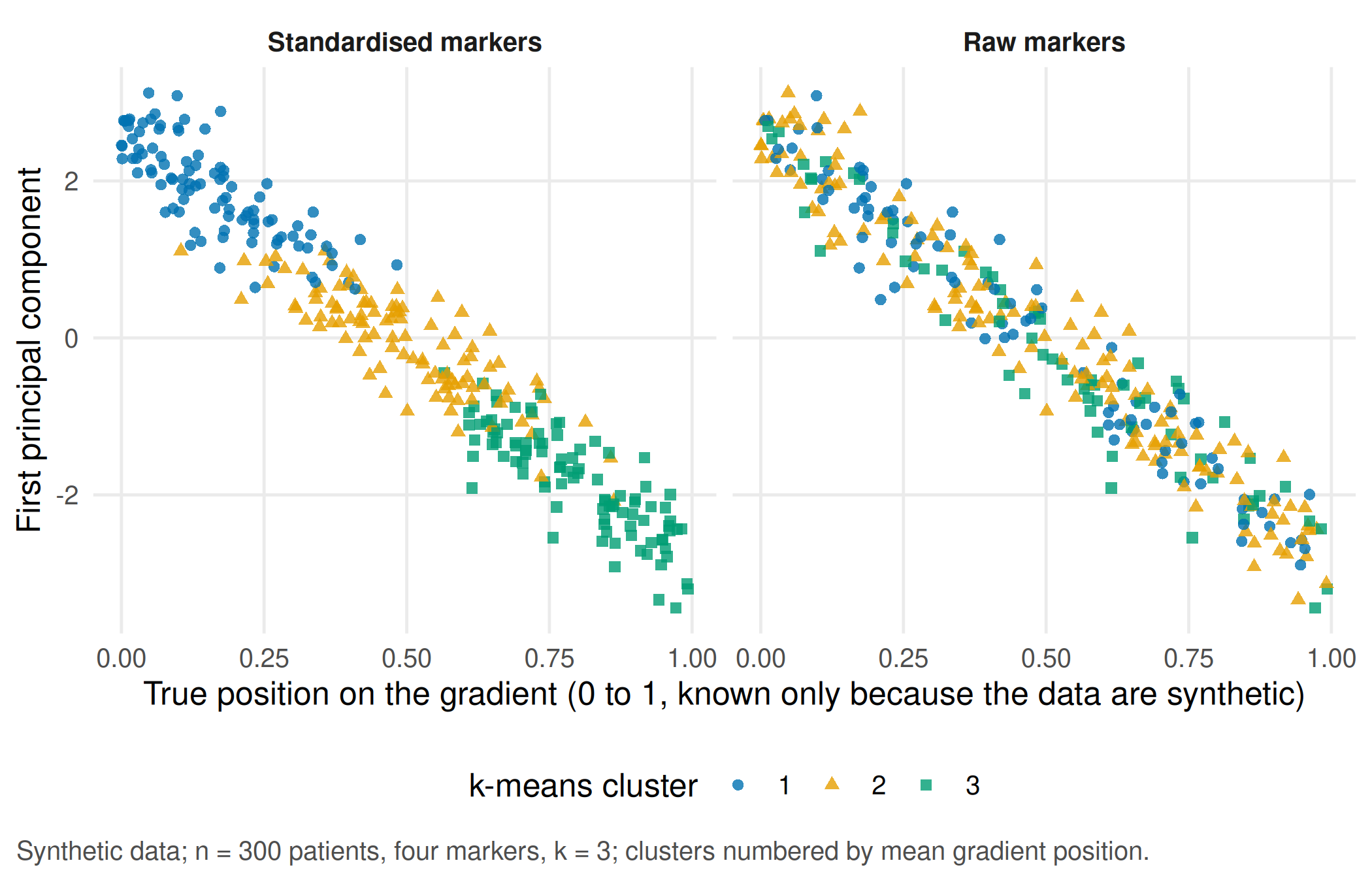
Report. The partitions on raw and standardised markers are unrelated (adjusted Rand index 0.05). The standardised clusters are slices of one gradient (rank correlation with the gradient 0.90), the separation is weak (mean silhouette width 0.30) and the bootstrap gives a median adjusted Rand index of 0.66. Even a perfectly stable split would not show that three distinct groups exist; a subtype label needs a consequence for patients and an external check, for example a different outcome or treatment response in an independent cohort.
TipCounter-check: predict first
Remove the unrelated marker and cluster the three gradient markers only. Will the clusters follow the gradient more closely or less closely?
# Counter-check: drop the unrelated marker and cluster the three gradient markers only
set.seed(1)
km_three <- kmeans(scale(markers[, c("marker_a", "marker_b", "marker_c")]), centers = 3, nstart = 25)
rho_three <- cor(order_by_gradient(km_three$cluster), gradient, method = "spearman")
rho_three
#> [1] 0.9160191stopifnot(rho_three > rho_scaled) # without the noise marker the clusters follow the gradient even more closelyStation 2 · A straight line or a flexible time function
Decision. The mixed model in Part B assumed a straight-line rise over 28 days. Is that good enough, or does the rise level off?
Assumption. A natural spline with three degrees of freedom lets the mean curve bend; both models keep the same random intercept and slope per person and are fitted by maximum likelihood so that their AIC can be compared.
# Part C, longitudinal station (unit 19): straight line versus natural spline for time, fitted by
# maximum likelihood on the observed data from Part B with the same random effects
fit_linear <- lmer(selenium ~ week * lesion + (1 + week | id), data = obs, REML = FALSE)
fit_spline <- lmer(selenium ~ ns(week, df = 3) * lesion + (1 + week | id), data = obs, REML = FALSE)
stopifnot(!isSingular(fit_linear), !isSingular(fit_spline))
aic_table <- data.frame(model = c("Linear time", "Natural spline, 3 df"),
                        parameters = c(attr(logLik(fit_linear), "df"), attr(logLik(fit_spline), "df")),
                        AIC = c(AIC(fit_linear), AIC(fit_spline)))
print(aic_table, digits = 4, row.names = FALSE)
#> model parameters AIC
#> Linear time 8 1138
#> Natural spline, 3 df 12 1127stopifnot(aic_table$AIC[2] < aic_table$AIC[1]) # the curvature is worth its extra parametersgrid <- expand.grid(week = seq(1, 28, by = 0.5) / 7, lesion = levels(obs$lesion))
grid$lesion <- factor(grid$lesion, levels = levels(obs$lesion))
curves <- rbind(data.frame(model = "Linear time", grid, fit = predict(fit_linear, grid, re.form = NA)),
data.frame(model = "Natural spline, 3 df", grid, fit = predict(fit_spline, grid, re.form = NA)))
obs_means <- aggregate(selenium ~ lesion + day, data = obs, FUN = mean)
p_spline <- ggplot() +
geom_line(data = curves, aes(week * 7, fit, colour = model, linetype = model), linewidth = 0.9) +
geom_point(data = obs_means, aes(day, selenium), colour = "black", size = 2) +
facet_wrap(~ lesion, labeller = labeller(lesion = c(complete = "Complete lesion", incomplete = "Incomplete lesion"))) +
scale_colour_manual(values = unname(cdsr_colours[c("orange", "blue")])) +
scale_linetype_manual(values = cdsr_linetypes[c(2, 1)]) +
scale_x_continuous(breaks = days) +
labs(x = "Day after injury", y = "Serum selenium (µg/L)", colour = NULL, linetype = NULL,
caption = sprintf("Synthetic data; n = 40 persons, %d observations. Points = observed means (day 28: completers only).", nrow(obs))) +
theme_cdsr()
show_figure(p_spline, "w5-spline.png")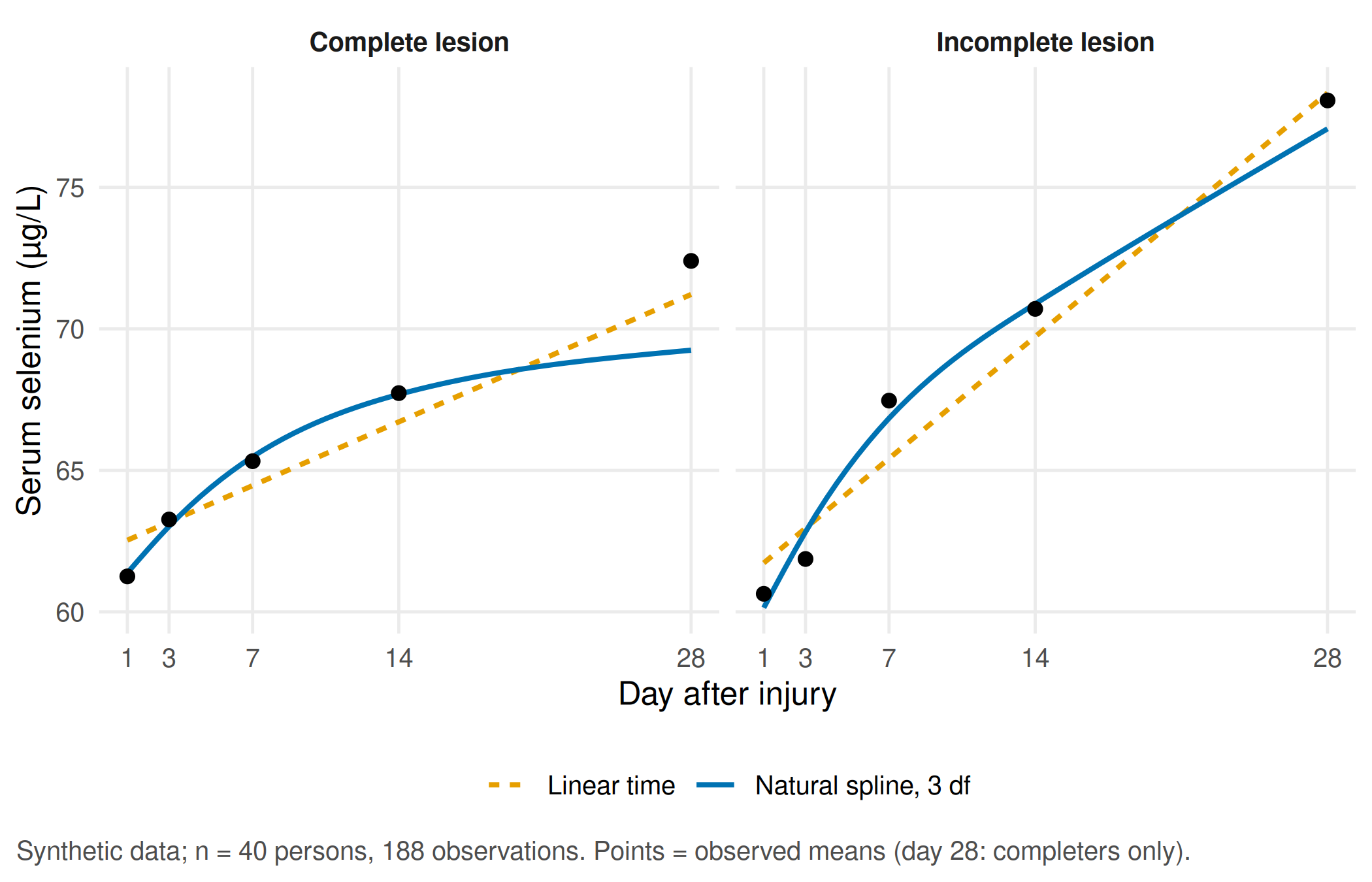
Report. The spline model has a lower AIC (1127 against 1138), so the rise levels off within four weeks and a single slope in µg/L per week summarises the trajectory only roughly. Note that the observed day-28 mean of the complete-lesion group lies above both curves: those are the completers from Part B, not a lack of fit.
Unit 20 · From a preclinical finding to the next experiment
Unit 20 is a reasoning task without code. Suppose a rodent model of spinal cord injury had shown a similar rise of the biomarker. Before proposing a further animal experiment, the group writes a one-page justification:
| Element | Question to answer |
|---|---|
| Hypothesis | Which single, testable statement would the next experiment decide? |
| Replacement | Could cell, tissue or in-silico models, or existing human data, answer it instead? |
| Reduction | Which unit is independent (animal, not sample), and how many animals does the effect size of interest need? Which design (blocking, repeated measures) reduces that number? |
| Refinement | Which procedures, endpoints and humane end points limit suffering? |
| Species and transfer | Why this species, and what would still be open for people after a positive result? |
| Criterion against a further experiment | Which result, or which existing evidence, would make the experiment unnecessary? |
| People affected | Which patients would benefit if the hypothesis holds, and what would they need to know? |
Use the NC3Rs description of the 3Rs and the reporting items of the ARRIVE guidelines 2.0 as checklists.
Your record for the workshop
- One sentence that states the target of Part A as either a causal estimand or a prognostic target, and a reason for every variable you would or would not adjust for.
- The Part B result with time unit, number of persons, number of observations, the interaction with its interval and the sensitivity finding.
- From your station in Part C: the alternative explanation and the plot or number that supports your conclusion.
- A draft of the one-page justification for unit 20 with one checkable alternative and one criterion against a further experiment.
Further reading
- Companion book: B02 · Describe, predict, explain and B13 · Longitudinal biomarkers – the required reading behind Parts A and B.
- Companion book: B14 · Cluster, gradient or artefact and B16 · Bayes, small samples and the 3Rs – background for station 1 and unit 20.
- Hernán, Hernández-Díaz and Robins (2004), A structural approach to selection bias – the collider argument of Part A in general form.
- CTTIR Courses: DAGs with dagitty and ggdag and MCAR, MAR, MNAR – drawing causal graphs and classifying missing data.
- CTTIR Courses: Linear mixed models with lme4 – random intercepts and slopes step by step.
- Methods in R: Random-Slope Models – model specification, diagnostics and reporting.
- Methods in R: k-Means Clustering and CTTIR Tutorials: Cluster Validation: Silhouette – what k-means optimises and how to judge separation.