R. Heller · Date: 2026-07-25 · Last changed: 2026-11-09
NoteAt a glance
Guiding question: Who will do something differently because of the output?
For: medical students, clinical researchers and doctoral candidates who are new to data analysis · Prerequisites: basic clinical knowledge; no programming experience
Ms K., 84 years old, falls in her kitchen early in the morning. She is a fictional patient. In the emergency department a hip radiograph is taken 30 minutes after arrival. Four minutes later, image-analysis software marks a possible femoral neck fracture. The radiologist reports 40 minutes after that, and the orthopaedic team plans surgery for the next morning. After the operation a nurse screens her for delirium, a physiotherapist gets her walking on the second postoperative day, and on day 5 a case manager decides whether to apply for geriatric rehabilitation. Every step produces information. This chapter asks a narrower question: which of these outputs changes what a named person does, and what happens when the output is wrong or missing?
A second, unrelated case runs alongside. A research group measures tissue oxygenation with hyperspectral imaging (HSI) in six rats after a standardised soft-tissue injury. They want to know whether the signal justifies a study in patients.
1.2 Core reading
Core reading · required for W1 · about 10 minutes · ends before ‘Lab’
1.2.1 An output is worth the action it changes
A test result, a risk score or a coloured box on an image is not useful in itself. It becomes useful when a person sees it in time, understands it and does something different from what they would otherwise have done. Fryback and Thornbury described this as a hierarchy for diagnostic imaging (Fryback and Thornbury 1991). Level 1 is technical image quality. Level 2 is diagnostic accuracy, such as sensitivity and specificity. Level 3 asks whether the information changes the clinician’s diagnostic thinking. Level 4 asks whether it changes the management plan, level 5 whether patients are better off, and level 6 whether the benefit justifies the costs to society. Each level is necessary for the next, but it does not guarantee it.
For Ms K. this hierarchy is concrete. Suppose the fracture flag is highly accurate (level 2). If the radiologist would have seen the same fracture 40 minutes later and the surgeon would have planned the same operation, nothing changes at level 4. The same flag can be valuable in a different setting: at night, when a junior doctor reads the image alone and might send a patient home with an undisplaced fracture. Accuracy belongs to the software. Decision value belongs to the software in a particular pathway.
1.2.2 The decision map
The simplest tool for this chapter is a decision map (Table 1.1). Each row is one output in Ms K.’s pathway. The columns force four answers: who acts, which action changes, in which population the output is meant to be used, and what happens when the output is wrong or unavailable. The last column, the fallback, is often forgotten. It describes how care continues if the software is switched off, gives no answer or gives a wrong one.
Table 1.1: Decision map for the fictional patient Ms K. (n = 1, synthetic case) and for the preclinical HSI study (n = 6 animals, synthetic). Each row names one output, the person who acts on it and the route back to usual care.
Output
Who acts differently
Changed action
Population
Harm if wrong
Fallback
Fracture flag on the hip radiograph
Emergency physician, radiologist
Second look; CT if the radiograph is equivocal
Adults with a fall and hip pain in the emergency department
Missed fracture: delayed surgery. False alarm: extra CT, time
Predicted need for inpatient rehabilitation on day 5
Case manager
Early application for geriatric rehabilitation
Inpatients after hip fracture surgery
Wrong placement; delayed discharge
Team discussion on the ward round
Gait speed in rehabilitation (m/s)
Physiotherapist
Adjust therapy; discuss discharge home
Patients in geriatric rehabilitation
Discharge too early or too late
Therapist’s clinical judgement
HSI oxygenation index in the rat model
Research team
Plan the next experiment, or stop
Rats in one injury model, not patients
Wasted animals and funding; premature human study
No clinical use; standard assessment continues
Three entries need particular care. The population is where the output was developed and checked, not where it might conceivably run. A fracture flag trained on emergency radiographs of adults says little about children or about follow-up images after surgery. The action must be specific. “Better decisions” is not an action; “request CT before discharge” is. The fallback must be a route that already works without the tool, so that a failure of the software does not become a failure of care.
The map rests on one assumption that is easy to overlook: the person in the ‘who acts’ column sees the output before the decision is taken, and has the time, the competence and the authority to act differently. If any of these conditions fails, accuracy is irrelevant. The Lab and the Counter-check below test the timing part of this assumption with a few lines of R.
1.2.3 From rat to patient: the translational chain
The HSI study looks similar but has a different addressee. Nobody treats a patient on the basis of six rats. The research team decides whether the signal deserves the next experiment. The output is a reason to formulate a hypothesis, not a reason to change care.
Between the two lies a chain of evidence. A preclinical signal must first be shown to be robust in animals: random allocation, blinded assessment and complete reporting, for which the ARRIVE guidelines give a checklist (Percie du Sert et al. 2020). Next comes feasibility in patients, then diagnostic accuracy in the target population, which STARD-AI helps to report (Sounderajah et al. 2025). Early clinical evaluation of a decision-support tool, with real users in a real workflow, is the subject of DECIDE-AI (Vasey et al. 2022). Only comparative studies can show that patients are better off. Each link answers a different question, and none can be skipped by a larger sample at an earlier link.
The chain often breaks. Van der Worp and colleagues cite a review of animal studies from leading high-impact journals: about one-third of the studies translated to the level of human randomised trials, and about one-tenth of the interventions were eventually approved for use in patients (published) (Worp et al. 2010). The same authors list typical reasons: weak internal validity (no randomisation, no blinding), limited external validity (young, otherwise healthy animals versus older patients with several diseases) and selective publication of positive results. Ms K. is 84 and takes several medicines. The rats are young, healthy and injured in a standardised way. That gap is not a flaw of the rat study. It is the reason why its result is a hypothesis.
1.2.4 Two teaching datasets that must stay apart
This book uses both cases repeatedly, so their data are kept strictly separate. The fracture cohort describes 12 fictional patients (identifiers P01 to P12; Ms K. is P01). Its unit of analysis is the patient. The HSI rat study describes six fictional animals (A1 to A6). It has thousands of rows, one per image pixel, but only six independent units. Mixing the two, or counting pixels as if they were animals, would produce numbers that look precise and mean nothing. Chapter 3 returns to this.
Question for the workshop: Choose one row of Table 1.1. At what time, and on which screen or sheet of paper, must the output appear so that the named person can still act on it? What would make the row worthless?
1.3 Lab
This Lab is the first contact with R. Every line is explained, and the expected output is printed below each command. You can follow the Lab on paper without running anything. If you want to run it, install R and RStudio first; CTTIR Course 1, Week 1 Session 2 shows the set-up step by step.
1.3.1 Step 1: R as a calculator
Text after # is a comment; R ignores it. The arrow <- stores a value under a name.
xray_min <-30# radiograph taken, minutes after arrivalflag_min <-34# fracture flag availablereport_min <-74# radiologist's report availablereport_min - flag_min # how many minutes earlier the flag arrives
#> [1] 40
The line starting with #> is R’s answer: the flag is available 40 minutes before the report. The [1] only means “first element of the result”.
1.3.2 Step 2: a table of Ms K.’s pathway
A table in R is called a data frame. Each column is a variable, each row an observation. Here one row is one step in Ms K.’s pathway.
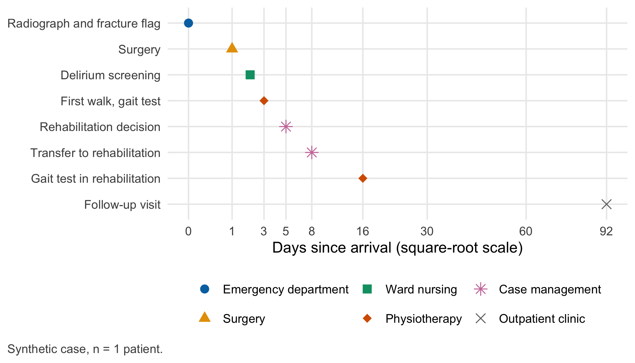
pathway <-data.frame(pid ="P01", # pseudonymous patient identifierstep =c("Radiograph and fracture flag", "Surgery", "Delirium screening","First walk, gait test", "Rehabilitation decision", "Transfer to rehabilitation","Gait test in rehabilitation", "Follow-up visit"),day =c(0, 1, 2, 3, 5, 8, 16, 92), # days since arrival (day 0 = arrival)role =c("Emergency department", "Surgery", "Ward nursing", "Physiotherapy","Case management", "Case management", "Physiotherapy", "Outpatient clinic"))pathway
#>   pid                         step day                 role
#> 1 P01 Radiograph and fracture flag   0 Emergency department
#> 2 P01                      Surgery   1              Surgery
#> 3 P01           Delirium screening   2         Ward nursing
#> 4 P01        First walk, gait test   3        Physiotherapy
#> 5 P01      Rehabilitation decision   5      Case management
#> 6 P01   Transfer to rehabilitation   8      Case management
#> 7 P01  Gait test in rehabilitation  16        Physiotherapy
#> 8 P01              Follow-up visit  92    Outpatient clinic
How to read this output:
The numbers 1 to 8 on the left are row numbers. R adds them; they are not data.
pid repeats the same value in every row. It is the identifier (ID) that links these rows to Ms K. in other tables. It is a pseudonym, not her name. In Chapter 3 the same ID appears in the gait-speed table.
day has a unit: days since arrival in the emergency department. This starting point is called time zero. A number without its unit and time zero cannot be checked by anyone else. Chapter 3 counts the same gait tests from the day of surgery (day 1 here), so the first test appears there as day 2, not day 3.
role names who acts. It is the column that the decision map is about.
Before we draw anything, R checks two facts about the table. stopifnot() stops with an error if a statement is false, so silence means “all true”.
stopifnot(nrow(pathway) ==8, # eight stepsall(diff(pathway$day) >=0)) # days never go backwards
1.3.3 Step 3: the first graphic
The package ggplot2 builds a graphic from three parts: the data, the mapping of columns to positions or colours (aes()), and the kind of mark (geom_point() for points). library() loads the package once per session.
library(ggplot2)pathway$step <-factor(pathway$step, levels =rev(pathway$step)) # keep the order top to bottompathway$role <-factor(pathway$role, levels =unique(pathway$role))ggplot(pathway, aes(x = day, y = step, colour = role, shape = role)) +geom_point(size =3) +scale_x_continuous(transform ="sqrt", breaks =c(0, 1, 3, 5, 8, 16, 30, 60, 92)) +scale_colour_manual(values =unname(cdsr_colours[c("blue", "orange", "green", "red", "purple", "grey")])) +scale_shape_manual(values =c(16, 17, 15, 18, 8, 4)) +labs(x ="Days since arrival (square-root scale)", y =NULL, colour =NULL, shape =NULL,caption ="Synthetic case, n = 1 patient.") +theme_cdsr() +guides(colour =guide_legend(nrow =2))
Figure 1.1: Pathway of the fictional patient Ms K. (P01) from the emergency department to the follow-up visit. Horizontal axis: days since arrival (day 0) on a square-root scale; one point per step, coloured by the role that acts. n = 1 patient, 8 steps; synthetic case.
TipWhat you should see
Eight points, one per row of the table, with the radiograph at the top left (day 0) and the follow-up visit at the bottom right (day 92). The first few days take up most of the width because the axis is drawn on a square-root scale; equal distances on the axis are therefore not equal numbers of days. Two pairs of points share a colour and shape: case management (days 5 and 8) and physiotherapy (days 3 and 16). If your figure shows fewer points, a row was lost; if the steps appear in alphabetical order, the factor() line was skipped.
1.3.4 Step 4: the decision map as data
The map in Table 1.1 can be stored as a data frame too. This makes a simple quality check possible: no cell may be empty, because an empty ‘fallback’ is exactly the gap that causes harm when software fails.
decision_map <-data.frame(output =c("Fracture flag", "Delirium score", "Rehabilitation prediction", "Gait speed", "HSI index"),who_acts =c("Emergency physician, radiologist", "Ward nurse", "Case manager", "Physiotherapist","Research team"),action =c("Second look; CT if equivocal", "Prevention bundle", "Early application","Adjust therapy", "Plan or stop next experiment"),population =c("Adults, fall, hip pain, ED", "Older inpatients after hip surgery","Inpatients after hip surgery", "Patients in geriatric rehabilitation", "Rats, one injury model"),fallback =c("Usual report", "Daily assessment", "Ward-round discussion", "Clinical judgement","No clinical use"))stopifnot(all(nzchar(as.matrix(decision_map)))) # nzchar = "not an empty string"table(clinical = decision_map$population !="Rats, one injury model")
#> clinical
#> FALSE  TRUE
#>     1     4
Four outputs concern patients and one concerns animals. The table() output counts them.
1.3.5 Step 5: two datasets, two units
The last step builds only the design of the two teaching datasets, without measured values, to show the difference between rows and independent units. expand.grid() creates every combination of its arguments.
The cohort has 60 rows for 12 patients; the rat study has 4,800 rows for six animals. The last check confirms that no identifier occurs in both datasets, so they cannot be merged by accident.
1.4 Counter-check
The key assumption of the decision map was timing. Suppose the hospital decides to run the fracture software as a nightly batch to save computing costs, so that the flag for Ms K. appears 18 hours after arrival instead of after 34 minutes. Before you run the code, predict: how many of the four emergency-department decisions below can the flag still influence?
ed_decisions <-data.frame(decision =c("Radiologist's report", "CT if radiograph equivocal", "Plan surgery", "Anaesthesia assessment"),hour =c(74, 80, 120, 150) /60# hours since arrival)flag_hour_now <-34/60# flag after 34 minutesflag_hour_batch <-18# nightly batch: 18 hoursed_decisions$flag_in_time_now <- flag_hour_now < ed_decisions$houred_decisions$flag_in_time_batch <- flag_hour_batch < ed_decisions$houred_decisions
With immediate processing the flag precedes all four decisions; as a nightly batch it precedes none. Its sensitivity and specificity are unchanged, yet its decision value for Ms K. falls to zero. The same logic applies to every row of Table 1.1: a delirium score that appears after the ward round, or a rehabilitation prediction delivered after the application deadline, cannot change the action it was built for.
1.5 Consequences for patients and operations
Patients. A missed fracture means pain, a second visit and delayed surgery; a false alarm means an extra CT, more radiation and more time in the emergency department. Both errors fall on the patient, but they are not equal, and the decision map makes the trade-off visible before any accuracy figure is discussed. Chapter 9 turns these errors into counts per shift, and Chapter 21 asks who carries them.
Operations. Every output needs a named owner and a fallback that works without it. If the fracture software fails at 3 a.m., the radiologist’s report remains the basis of care. A tool whose failure goes unnoticed is more dangerous than no tool, because staff may rely on a silence that only means “not processed”. Monitoring and stopping rules are the subject of Chapter 20.
Regulation. Whether fracture-flagging software is a medical device depends on its intended purpose, as set by the manufacturer, under the EU Medical Device Regulation (MDR, Regulation (EU) 2017/745) (European Parliament and Council of the European Union 2017). Annex VIII, Rule 11 of this binding text classifies software that provides information used for diagnostic or therapeutic decisions. In which class a given product falls, and which obligations of the EU Artificial Intelligence Act (Regulation (EU) 2024/1689, amended by Regulation (EU) 2026/1744) apply from which date (European Parliament and Council of the European Union 2024, 2026), is worked through in Chapter 22 (status: November 2026). A research prototype that is quietly used for patient care changes its regulatory position; that is a question for the institution, not for the analyst alone (open, to be clarified locally with the regulatory affairs or medical device officer).
Animal research. The rat study is subject to Directive 2010/63/EU on the protection of animals used for scientific purposes (European Parliament and Council of the European Union 2010), published on 20 October 2010 and in force since 9 November 2010. Its Article 4 obliges Member States to ensure replacement, reduction and refinement (the 3Rs) wherever possible; the national implementing provisions apply from 1 January 2013. Which national authority approves a given project is a local question (open, to be clarified with the institution’s animal welfare body). ARRIVE 2.0 governs how the study is reported (Percie du Sert et al. 2020), and the NC3Rs explain the 3Rs for planning (NC3Rs 2026). A within-animal control limb, as in our design, is one way to reduce animal numbers, but it does not replace a justified sample size (Chapter 16).
Data protection. Not directly touched here, because all data are synthetic. It becomes relevant as soon as real radiographs or registry data leave the treating hospital (Chapter 23).
1.6 Look up and transfer
Reviewer question: For the output you evaluate, which named role changes which action, at what time after time zero, in which population — and what is the fallback when the output is missing or wrong?
Self-test: A model predicts on day 7 after hip surgery whether a patient will need inpatient rehabilitation. In the hospital, rehabilitation applications must be submitted by day 5. The model’s discrimination is good. What is its decision value in this pathway, and what would you change first: the model, its timing or its addressee?
TipAnswer
As deployed, the decision value is zero: the output arrives after the decision it is meant to inform. Improving the model’s accuracy does not help. The first change is the timing (predict on day 3 or 4 with the information then available, which may lower accuracy) or the addressee (use the prediction for a later decision, such as the timing of discharge from rehabilitation). Fryback and Thornbury’s levels 3 and 4 are not reached, whatever level 2 shows.
Annotated sources:
Fryback and Thornbury (1991) — the hierarchy from technical quality to societal value; the basis for separating accuracy from decision value in this chapter.
Worp et al. (2010) — reasons why animal findings fail to translate, with the published estimate quoted in the Core reading.
Percie du Sert et al. (2020) — ARRIVE 2.0, the reporting checklist for the rat study.
Sounderajah et al. (2025) — STARD-AI, reporting of diagnostic accuracy studies of AI tools (level 2).
Vasey et al. (2022) — DECIDE-AI, reporting of early clinical evaluation in real workflows (levels 3 and 4).
European Parliament and Council of the European Union (2010) — the binding EU basis for the 3Rs (Article 4).
1.7 Further reading
Chapter 2 — the same pathway seen as three different questions: describe, predict, explain.
Chapter 9 — what the fracture flag means in counts of alarms per shift at different prevalences.
Chapter 19 — when a result from one centre or one species may be transferred to the next.
European Parliament and Council of the European Union. 2010. Directive 2010/63/EU of 22 September 2010 on the Protection of Animals Used for Scientific Purposes. https://eur-lex.europa.eu/eli/dir/2010/63/oj/eng.
European Parliament and Council of the European Union. 2024. Regulation (EU) 2024/1689 Laying down Harmonised Rules on Artificial Intelligence (Artificial Intelligence Act). https://eur-lex.europa.eu/eli/reg/2024/1689/oj.
European Parliament and Council of the European Union. 2026. Regulation (EU) 2026/1744 Amending Regulation (EU) 2024/1689 (Digital Omnibus on AI). https://eur-lex.europa.eu/eli/reg/2026/1744/oj.
Fryback, Dennis G., and John R. Thornbury. 1991. “The Efficacy of Diagnostic Imaging.”Medical Decision Making 11 (2): 88–94. https://doi.org/10.1177/0272989X9101100203.
Percie du Sert, Nathalie, Viki Hurst, Amrita Ahluwalia, et al. 2020. “The ARRIVE Guidelines 2.0: Updated Guidelines for Reporting Animal Research.”PLOS Biology 18 (7): e3000410. https://doi.org/10.1371/journal.pbio.3000410.
Sounderajah, Viknesh, Ahmad Guni, Xiaoxuan Liu, et al. 2025. “The STARD-AI Reporting Guideline for Diagnostic Accuracy Studies Using Artificial Intelligence.”Nature Medicine 31: 3283–89. https://doi.org/10.1038/s41591-025-03953-8.
Vasey, Baptiste, Myura Nagendran, Bruce Campbell, et al. 2022. “Reporting Guideline for the Early Stage Clinical Evaluation of Decision Support Systems Driven by Artificial Intelligence: DECIDE-AI.”BMJ 377: e070904. https://doi.org/10.1136/bmj-2022-070904.
Worp, H. Bart van der, David W. Howells, Emily S. Sena, et al. 2010. “Can Animal Models of Disease Reliably Inform Human Studies?”PLoS Medicine 7 (3): e1000245. https://doi.org/10.1371/journal.pmed.1000245.