library(ggplot2)
library(class) # k-nearest-neighbour classifier knn()Lab W4 · Spectra, image split and animal split
Teaching units 13–15: a spectral index under changing light, an image split against an animal split, and two elective stations on gait angles and tissue phenotypes.
Everyone works through Parts A and B, the shared hyperspectral imaging lab. Part C offers two elective stations, gait and tissue; each group chooses one and presents its finding to a group from the other station in unit 16. Every part follows the same five steps: state the decision, look at the data, name the assumption, compute in R and write one sentence for the person who has to act.
All animals, persons and tissue classes are fictitious and all numbers are synthetic or teaching assumptions. The classes A and B stand for any two tissue states a research group might want to separate; they describe no real tissue, device or study. If R is new to you, read the code and the printed output first and answer the questions on paper. If you are fluent in R, try the extra counter-checks.
Part A · A spectral index under changing light (unit 13)
Decision. A research group wants to use a simple spectral index as a baseline for separating tissue class A from class B in hyperspectral images of fictitious animals. Before anyone trains a learning model, the group has to know what else moves the index.
Look at the data. Six animals (three per class) contribute five reflectance spectra each, from 500 to 1,000 nm in 10 nm steps. Reflectance is the share of light returned by the tissue, between 0 and 1.
# Part A (unit 13): synthetic reflectance spectra, 500-1000 nm in 10 nm steps
wavelength <- seq(500, 1000, by = 10)                        # nm
# One reflectance spectrum (0-1) for a tissue class, with an animal-specific gain and offset
make_spectrum <- function(class, gain, offset, noise_sd) {
  base    <- 0.25 + 0.30 * plogis((wavelength - 690) / 25)  # rise towards the near infrared
  dip_vis <- ifelse(class == "A", 0.10, 0.05) * exp(-((wavelength - 560) / 25)^2)
  dip_nir <- ifelse(class == "A", 0.02, 0.06) * exp(-((wavelength - 760) / 20)^2)
  gain * (base - dip_vis - dip_nir) + offset + rnorm(length(wavelength), 0, noise_sd)
}
# Normalised difference index of two bands: (R800 - R560) / (R800 + R560)
nd_index <- function(r) {
  r800 <- r[wavelength == 800]
  r560 <- r[wavelength == 560]
  (r800 - r560) / (r800 + r560)
}

set.seed(20260413)
animals_a <- data.frame(id = sprintf("AN%02d", 1:6), class = rep(c("A", "B"), each = 3),
                        gain = rnorm(6, 1, 0.04), offset = rnorm(6, 0, 0.01))
spectra_a <- do.call(rbind, lapply(seq_len(nrow(animals_a)), function(i) {
  a <- animals_a[i, ]
  do.call(rbind, lapply(1:5, function(s) {
    data.frame(id = a$id, class = a$class, spectrum = s, wavelength = wavelength,
               reflectance = make_spectrum(a$class, a$gain, a$offset, noise_sd = 0.004))
  }))
}))
# One row per spectrum with its index
index_a <- aggregate(reflectance ~ id + class + spectrum, data = spectra_a, FUN = nd_index)
names(index_a)[names(index_a) == "reflectance"] <- "nd_index"
stopifnot(length(unique(spectra_a$id)) == 6, nrow(index_a) == 30)
aggregate(nd_index ~ class, data = index_a, FUN = function(x) round(mean(x), 3))
#> class nd_index
#> 1 A 0.567
#> 2 B 0.449mean_spectra <- aggregate(reflectance ~ id + class + wavelength, data = spectra_a, FUN = mean)
p_spectra <- ggplot(mean_spectra, aes(wavelength, reflectance, group = id, colour = class, linetype = class)) +
geom_vline(xintercept = c(560, 800), colour = "grey60", linetype = "22") +
geom_line(linewidth = 0.7) +
annotate("text", x = c(560, 800), y = 0.08, label = c("560 nm", "800 nm"), hjust = -0.1, size = 3.2,
colour = "grey35") +
scale_colour_manual(values = unname(cdsr_colours[c("blue", "orange")])) +
scale_linetype_manual(values = cdsr_linetypes[1:2]) +
coord_cartesian(ylim = c(0.05, 0.6)) +
labs(x = "Wavelength (nm)", y = "Reflectance (0-1, unitless)", colour = "Tissue class",
linetype = "Tissue class",
caption = "Synthetic data: mean of 5 spectra per animal; n = 6 fictitious animals (3 per class). Dashed lines: index bands.") +
theme_cdsr()
show_figure(p_spectra, "w4-spectra.png")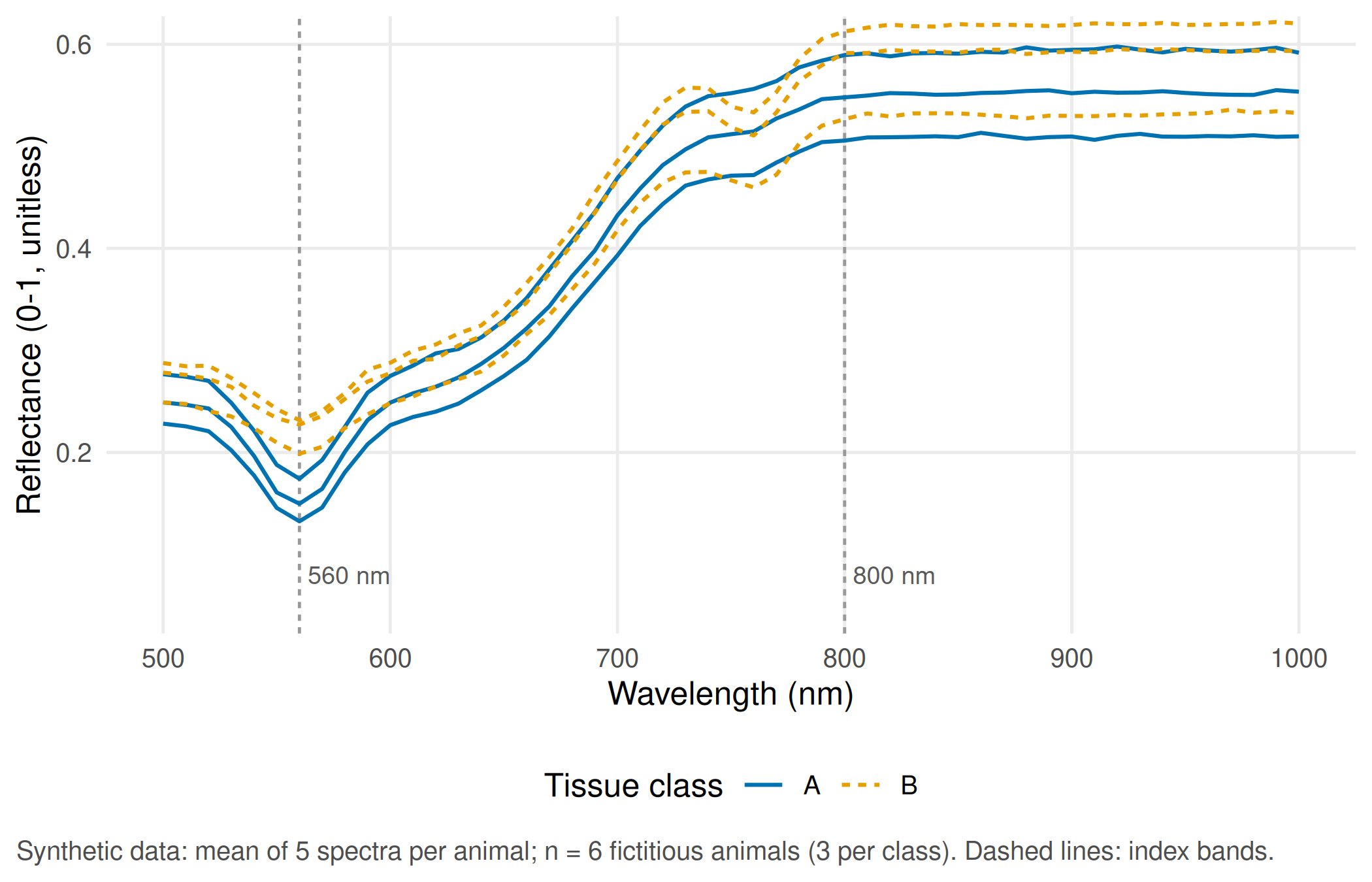
The index compares the two marked bands: (R800 − R560) / (R800 + R560). In this synthetic set its mean is 0.567 for class A and 0.449 for class B.
Assumption. The index measures tissue, not the lamp. We test this with two changes of illumination: a lamp that is 20% weaker at every wavelength, and a lamp with a different colour balance (a linear tilt that weakens green and strengthens near-infrared light). The proposed reference measurement is a white and a dark reference recorded under the same lamp: the camera records counts, and reflectance is computed as (counts − dark) / (white − dark).
TipCounter-check: predict first
Will the weaker lamp change the index? Will the tilted lamp make class B look more like class A or less? Write down your guesses before you run the next chunk.
# Two changes of illumination applied to every spectrum
brightness <- function(r) 0.8 * r                                    # lamp 20% weaker, same colour
tilt       <- function(r) r * (1 + 0.3 * (wavelength - 750) / 250)    # lamp with a different colour balance
# White and dark reference: the camera records counts, not reflectance
camera_counts <- function(r, lamp) 120 + 3000 * lamp * r              # dark current 120 counts, gain 3000
lamp_tilted   <- 1 + 0.3 * (wavelength - 750) / 250
correct_with_reference <- function(counts, lamp) {
  dark  <- camera_counts(0, lamp)                                     # shutter closed
  white <- camera_counts(1, lamp)                                     # white standard, reflectance 1
  (counts - dark) / (white - dark)
}
illum <- do.call(rbind, lapply(split(spectra_a, list(spectra_a$id, spectra_a$spectrum), drop = TRUE),
  function(d) {
    r <- d$reflectance
    data.frame(id = d$id[1], class = d$class[1], spectrum = d$spectrum[1],
               original = nd_index(r), brighter_lamp_off = nd_index(brightness(r)),
               tilted_lamp = nd_index(tilt(r)),
               tilted_lamp_corrected = nd_index(correct_with_reference(camera_counts(r, lamp_tilted),
                                                                       lamp_tilted)))
  }))
class_gap  <- diff(tapply(illum$original, illum$class, mean))        # B minus A, original lamp
tilt_shift <- mean(illum$tilted_lamp - illum$original)
round(c(class_gap = unname(class_gap), tilt_shift = tilt_shift), 3)
#> class_gap tilt_shift
#> -0.117 0.108stopifnot(
max(abs(illum$brighter_lamp_off - illum$original)) < 1e-12, # index ignores overall brightness
abs(tilt_shift) > abs(class_gap) / 2, # a colour shift moves it by more than half the class gap
max(abs(illum$tilted_lamp_corrected - illum$original)) < 1e-10 # white/dark reference restores it
)illum_long <- data.frame(
id = rep(illum$id, 4), class = rep(illum$class, 4),
condition = factor(rep(c("Original lamp", "Lamp 20% weaker", "Lamp with colour tilt",
"Tilt + white/dark reference"), each = nrow(illum)),
levels = c("Original lamp", "Lamp 20% weaker", "Lamp with colour tilt",
"Tilt + white/dark reference")),
nd_index = c(illum$original, illum$brighter_lamp_off, illum$tilted_lamp, illum$tilted_lamp_corrected)
)
illum_animal <- aggregate(nd_index ~ id + class + condition, data = illum_long, FUN = mean)
p_illum <- ggplot(illum_animal, aes(condition, nd_index, colour = class, shape = class)) +
geom_point(size = 2.6, position = position_jitter(width = 0.08, height = 0, seed = 1)) +
scale_colour_manual(values = unname(cdsr_colours[c("blue", "orange")])) +
scale_shape_manual(values = cdsr_shapes[1:2]) +
scale_x_discrete(labels = function(x) gsub(" ", "\n", sub(" \\+ ", " +\n", x))) +
labs(x = NULL, y = "Index (R800 - R560) / (R800 + R560)", colour = "Tissue class", shape = "Tissue class",
caption = "Synthetic data: each point is the mean of 5 spectra of one animal; n = 6 fictitious animals.") +
theme_cdsr()
show_figure(p_illum, "w4-illumination.png")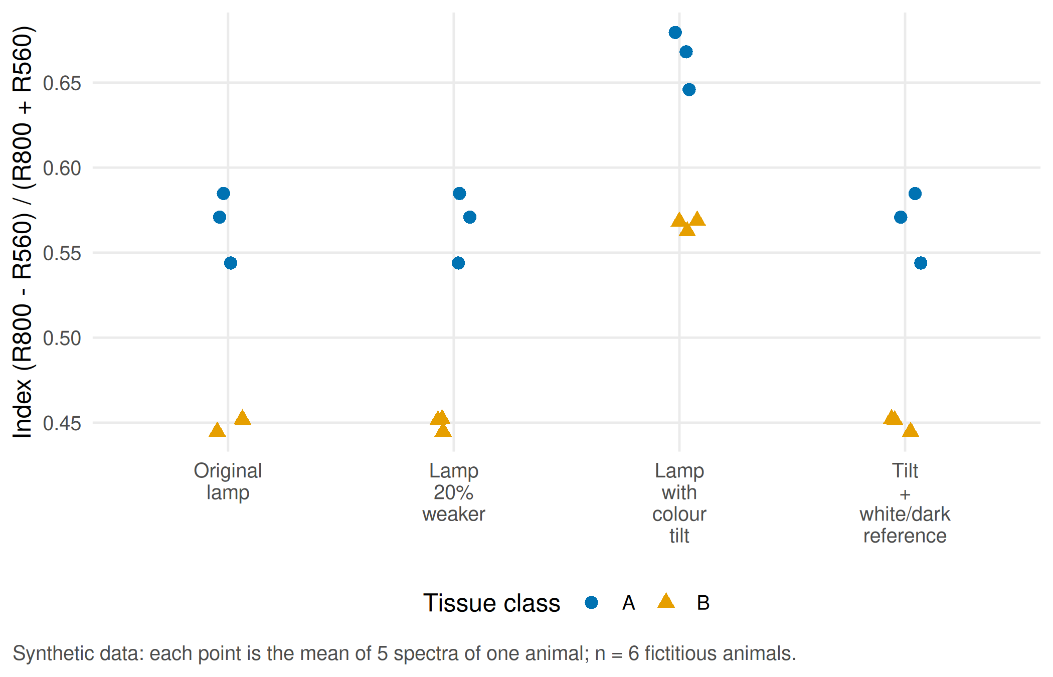
Report. A uniformly weaker lamp leaves the index unchanged, because it cancels in the ratio. A change in the lamp’s colour balance shifts the index by 0.108 on average, about as much as the difference between the classes (0.117). If class B animals were imaged under a different lamp than class A animals, the lamp alone could create or erase the class difference: illumination is a confounder of the tissue comparison. The white/dark reference recorded under the same lamp removes the effect completely in this simulation; in practice it has to be recorded for every session and documented in the model passport.
Part B · Image split against animal split (unit 14)
Decision. A reviewer asks whether the reported accuracy describes new spectra of known animals or new animals. These are two different target statements, and they need two different test plans.
Look at the data. Four fictitious animals contribute three spectra each. Classes belong to animals: AN1 and AN2 are class A, AN3 and AN4 class B.
# Part B (unit 14): four fictitious animals with three spectra each; classes belong to animals
set.seed(20260414)
four <- data.frame(id = rep(c("AN1", "AN2", "AN3", "AN4"), each = 3),
                   spectrum = rep(1:3, times = 4),
                   class = rep(c("A", "A", "B", "B"), each = 3))
four$nd_index <- round(sapply(seq_len(nrow(four)), function(i)
  nd_index(make_spectrum(four$class[i], gain = 1, offset = 0, noise_sd = 0.004))), 3)
four
#> id spectrum class nd_index
#> 1 AN1 1 A 0.564
#> 2 AN1 2 A 0.559
#> 3 AN1 3 A 0.580
#> 4 AN2 1 A 0.564
#> 5 AN2 2 A 0.559
#> 6 AN2 3 A 0.571
#> 7 AN3 1 B 0.464
#> 8 AN3 2 B 0.467
#> 9 AN3 3 B 0.453
#> 10 AN4 1 B 0.468
#> 11 AN4 2 B 0.463
#> 12 AN4 3 B 0.465Assumption. To isolate the data leak, we use a deliberately trivial baseline instead of a real model: for a known animal it returns the class already seen for that animal; for an unknown animal it returns the default class A, fixed before the test.
# Deliberately trivial baseline: return the class already seen for a known animal;
# for an animal not seen in training, return the pre-specified default class A
predict_lookup <- function(train, test, default = "A") {
  seen <- tapply(train$class, train$id, function(x) names(which.max(table(x))))
  ifelse(test$id %in% names(seen), seen[test$id], default)
}
evaluate_split <- function(train, test, aim, split) {
  test$predicted <- predict_lookup(train, test)
  test$correct <- test$predicted == test$class
  per_animal <- tapply(test$correct, test$id, all)
  data.frame(aim = aim, split = split,
             shared_ids = length(intersect(unique(train$id), unique(test$id))),
             correct_spectra = sum(test$correct), test_spectra = nrow(test),
             correct_animals = sum(per_animal), test_animals = length(per_animal))
}
# Image split: two spectra per animal in training, the third in the test set
image_train <- four[four$spectrum <= 2, ]
image_test  <- four[four$spectrum == 3, ]
# Animal split: AN1 (class A) and AN3 (class B) in training; AN2 (A) and AN4 (B) are new animals
animal_train <- four[four$id %in% c("AN1", "AN3"), ]
animal_test  <- four[four$id %in% c("AN2", "AN4"), ]
split_results <- rbind(
  evaluate_split(image_train, image_test, "Another spectrum of a known animal", "Image split"),
  evaluate_split(animal_train, animal_test, "Spectra of two new animals", "Animal split"))
split_results
#> aim split shared_ids correct_spectra
#> 1 Another spectrum of a known animal Image split 4 4
#> 2 Spectra of two new animals Animal split 0 3
#> test_spectra correct_animals test_animals
#> 1 4 4 4
#> 2 6 1 2intersect(unique(animal_train$id), unique(animal_test$id)) # must be empty#> character(0)# Target values of the teaching case
stopifnot(
split_results$correct_spectra[1] == 4, split_results$test_spectra[1] == 4,
split_results$shared_ids[1] == 4, # image split: every test animal is known
split_results$correct_spectra[2] == 3, split_results$test_spectra[2] == 6,
split_results$correct_animals[2] == 1, split_results$test_animals[2] == 2,
length(intersect(unique(animal_train$id), unique(animal_test$id))) == 0
)Report. In the image split, every test animal also appears in training, and the lookup solves 4/4 test spectra without knowing anything about tissue: it measures recognition of animals. In the animal split, the intersection of animal identifiers is empty, the default class solves 3/6 spectra and 1/2 animals. The independent denominator is two animals, not six spectra.
TipCounter-check: predict first
The default class for unknown animals changes from A to B. How many spectra and how many animals will the lookup now classify correctly in the animal split?
# Counter-check: the pre-specified default class for unknown animals becomes B instead of A
pred_b <- predict_lookup(animal_train, animal_test, default = "B")
countercheck <- c(correct_spectra = sum(pred_b == animal_test$class),
                  correct_animals = sum(tapply(pred_b == animal_test$class, animal_test$id, all)))
countercheck
#> correct_spectra correct_animals
#> 3 1stopifnot(countercheck[["correct_spectra"]] == 3, countercheck[["correct_animals"]] == 1)The count stays the same, but a different animal is now correct. With two test animals, any result is fragile.
Extension: a nearest-neighbour model on twelve animals
The same leak affects real models. Twelve fictitious animals (six per class) contribute ten spectra each. In this simulation the differences between animals are larger than the difference between the classes. A 1-nearest-neighbour model is evaluated twice: once with spectra assigned to ten folds at random, once leaving one whole animal out at a time, using the same animal identifiers.
# Extension: 12 fictitious animals x 10 spectra; animal-specific signatures are stronger than the class signal
set.seed(20260415)
animals_b <- data.frame(id = sprintf("AN%02d", 21:32), class = rep(c("A", "B"), each = 6),
                        gain = rnorm(12, 1, 0.08), offset = rnorm(12, 0, 0.03))
spectra_b <- t(sapply(rep(seq_len(12), each = 10), function(i)
  make_spectrum(animals_b$class[i], animals_b$gain[i], animals_b$offset[i], noise_sd = 0.015)))
meta_b <- data.frame(id = rep(animals_b$id, each = 10), class = rep(animals_b$class, each = 10),
                     spectrum = rep(1:10, times = 12))
# Cross-validated 1-nearest-neighbour predictions for a given fold assignment
cv_knn <- function(fold) {
  pred <- character(nrow(meta_b))
  overlap <- integer(0)
  for (f in sort(unique(fold))) {
    test_rows <- fold == f
    pred[test_rows] <- as.character(knn(spectra_b[!test_rows, ], spectra_b[test_rows, , drop = FALSE],
                                        cl = factor(meta_b$class[!test_rows]), k = 1))
    overlap <- c(overlap, length(intersect(meta_b$id[!test_rows], meta_b$id[test_rows])))
  }
  list(pred = pred, overlap = overlap)
}
fold_spectrum <- sample(rep(1:10, length.out = nrow(meta_b)))    # spectra assigned to folds at random
fold_animal   <- as.integer(factor(meta_b$id))                    # leave one animal out
cv_s <- cv_knn(fold_spectrum)
cv_a <- cv_knn(fold_animal)
meta_b$correct_spectrum_split <- cv_s$pred == meta_b$class
meta_b$correct_animal_split   <- cv_a$pred == meta_b$class
knn_summary <- data.frame(
  split = c("Spectrum-wise 10-fold", "Animal-wise (leave one animal out)"),
  folds_sharing_animals = c(sum(cv_s$overlap > 0), sum(cv_a$overlap > 0)),
  correct_spectra = c(sum(meta_b$correct_spectrum_split), sum(meta_b$correct_animal_split)),
  spectra = nrow(meta_b),
  animals_majority_correct = c(sum(tapply(meta_b$correct_spectrum_split, meta_b$id, mean) > 0.5),
                               sum(tapply(meta_b$correct_animal_split, meta_b$id, mean) > 0.5)),
  animals = 12)
knn_summary
#> split folds_sharing_animals correct_spectra
#> 1 Spectrum-wise 10-fold 10 117
#> 2 Animal-wise (leave one animal out) 0 64
#> spectra animals_majority_correct animals
#> 1 120 12 12
#> 2 120 6 12stopifnot(
all(cv_a$overlap == 0), # no animal in training and test at once
sum(cv_s$overlap > 0) == 10, # every random fold shares animals
knn_summary$correct_spectra[1] > knn_summary$correct_spectra[2] + 20 # random split looks clearly better
)per_animal <- data.frame(
id = rep(animals_b$id, 2), class = rep(animals_b$class, 2),
split = factor(rep(c("Spectrum-wise split", "Animal-wise split"), each = 12),
levels = c("Spectrum-wise split", "Animal-wise split")),
accuracy = c(tapply(meta_b$correct_spectrum_split, meta_b$id, mean)[animals_b$id],
tapply(meta_b$correct_animal_split, meta_b$id, mean)[animals_b$id]))
# spread the 12 animals slightly along the x axis so that overlapping points stay visible
per_animal$x <- as.integer(per_animal$split) + (as.integer(factor(per_animal$id)) - 6.5) * 0.025
p_knn <- ggplot(per_animal, aes(x, accuracy, group = id)) +
geom_line(colour = "grey75") +
geom_point(aes(colour = class, shape = class), size = 2.6) +
scale_colour_manual(values = unname(cdsr_colours[c("blue", "orange")])) +
scale_shape_manual(values = cdsr_shapes[1:2]) +
scale_x_continuous(breaks = 1:2, labels = levels(per_animal$split)) +
scale_y_continuous(labels = scales::percent, limits = c(0, 1)) +
labs(x = NULL, y = "Spectra correct per animal", colour = "Tissue class",
shape = "Tissue class",
caption = "Synthetic data, 1-nearest-neighbour model; n = 12 fictitious animals (independent units), 10 spectra each.") +
theme_cdsr()
show_figure(p_knn, "w4-knn-split.png")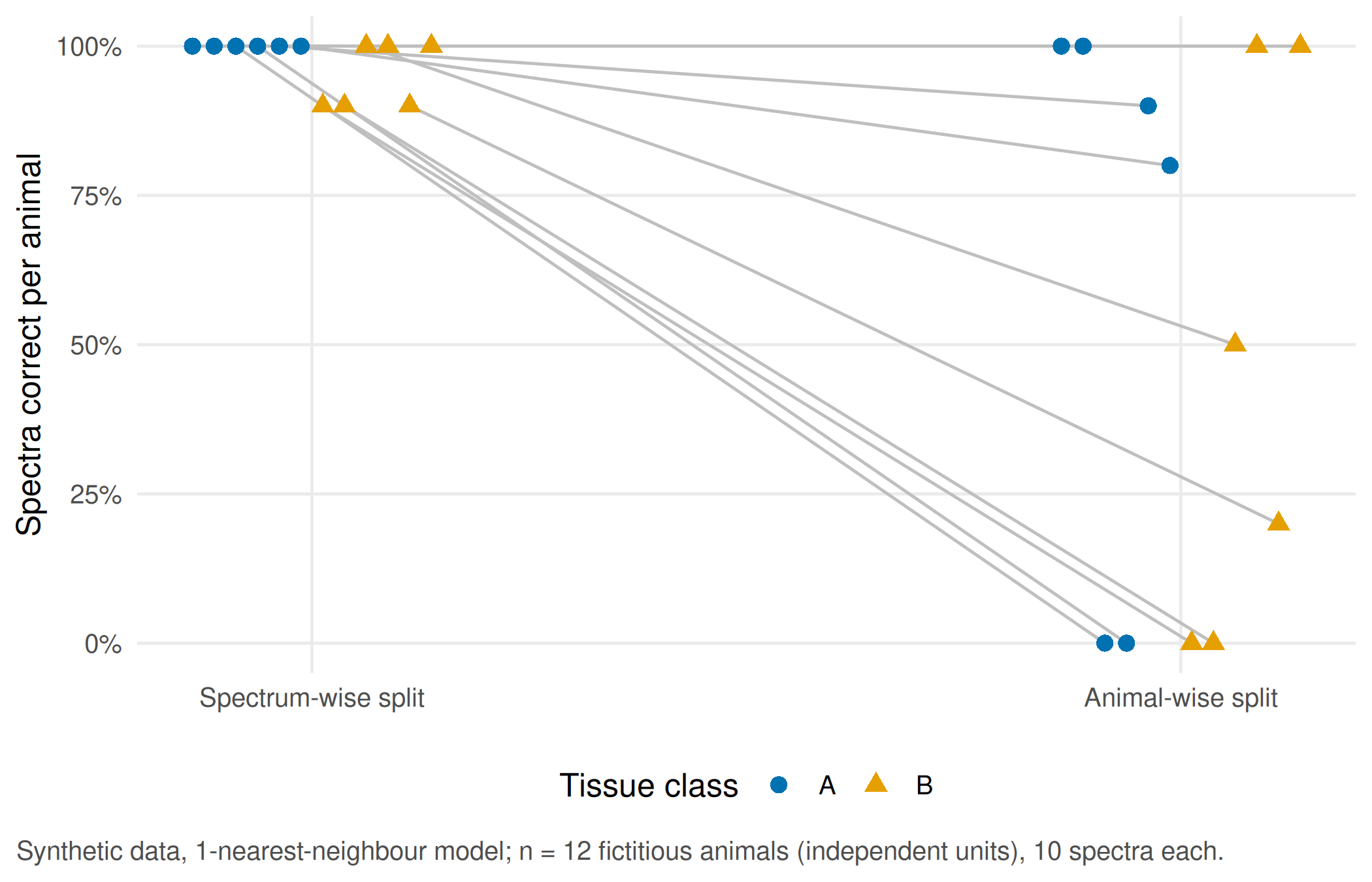
Report. With spectra split at random, every fold shares animals with its training data and the model classifies 117/120 spectra correctly. Leaving whole animals out, it manages 64/120 spectra and a majority of spectra for 6/12 animals. The model has mostly learnt which animal a spectrum came from. Even the animal-wise result only supports a statement about new animals of the same fictitious species under the same imaging set-up; a statement about patients needs a new study in the target population.
WarningCommon mistake
Reporting “120 test spectra” as the sample size. Spectra of one animal are not independent observations (pseudoreplication, see Lazic 2010). The unit that can be generalised is the animal; report the number of animals in training and test and check that the intersection of their identifiers is empty.
NoteOther implementation: Python/scikit-learn
If an existing image model is written in Python, grouped folds can be built in the same pipeline with scikit-learn GroupKFold, using the animal identifier as the group. The concrete advantage is that the split, pre-processing and model stay in one workflow and cannot drift apart. For a fair comparison with this lab, the input table, the animal identifiers, the metric and the unit of reporting must be identical; the shared target value is zero shared identifiers per fold, while the order of folds may differ. For image models with pretrained networks, scikit-image and the PyTorch transfer-learning tutorial document the pre-processing and weights that would have to be fixed as well. Status: conceptual comparison, not run.
Part C · Elective stations (unit 15)
Choose one station. Both end with a figure that states its unit and the independent sample size, and with one realistic consequence of the measurement error you found.
Station gait: one angle, two cameras, two methods
Decision. A rehabilitation team considers replacing a marker-based reference measurement of knee flexion with a video method. They need to know whether the two methods are similar enough for their decision.
Look at the data. The knee angle is computed from three landmarks: hip, knee and ankle. For a single synthetic leg with a true knee flexion of 40 degrees, we turn the camera away from the side view.
# Part C, gait station (unit 15): knee flexion from three 2D landmarks
knee_flexion <- function(hip, knee, ankle) {
  u <- hip - knee
  v <- ankle - knee
  inner <- acos(sum(u * v) / sqrt(sum(u^2) * sum(v^2))) * 180 / pi    # angle at the knee, degrees
  180 - inner                                                       # 0 = straight leg
}
# A leg in the sagittal plane: thigh 0.45 m tilted 20 degrees forward, true knee flexion 40 degrees
deg <- pi / 180
hip   <- c(0, 0.90)
knee  <- hip + 0.45 * c(sin(20 * deg), -cos(20 * deg))
ankle <- knee + 0.42 * c(sin(-20 * deg), -cos(-20 * deg))
# Camera turned away from the side view by theta: horizontal distances shrink by cos(theta)
perspective <- data.frame(camera_deg = seq(0, 45, by = 5))
perspective$measured <- sapply(perspective$camera_deg, function(th) {
  squeeze <- c(cos(th * deg), 1)
  knee_flexion(hip * squeeze, knee * squeeze, ankle * squeeze)
})
round(perspective, 1)
#> camera_deg measured
#> 1 0 40.0
#> 2 5 39.9
#> 3 10 39.4
#> 4 15 38.7
#> 5 20 37.8
#> 6 25 36.5
#> 7 30 35.0
#> 8 35 33.2
#> 9 40 31.2
#> 10 45 28.9stopifnot(isTRUE(all.equal(perspective$measured[1], 40)),
perspective$measured[perspective$camera_deg == 30] < 40)p_persp <- ggplot(perspective, aes(camera_deg, measured)) +
geom_hline(yintercept = 40, linetype = "22", colour = "grey50") +
geom_line(colour = cdsr_colours[["blue"]]) +
geom_point(colour = cdsr_colours[["blue"]], shape = cdsr_shapes[1]) +
labs(x = "Camera rotation away from the side view (degrees)", y = "Measured knee flexion (degrees)",
caption = "Synthetic geometry of one leg with true knee flexion 40 degrees (dashed line); 2D projection only.") +
theme_cdsr()
show_figure(p_persp, "w4-perspective.png")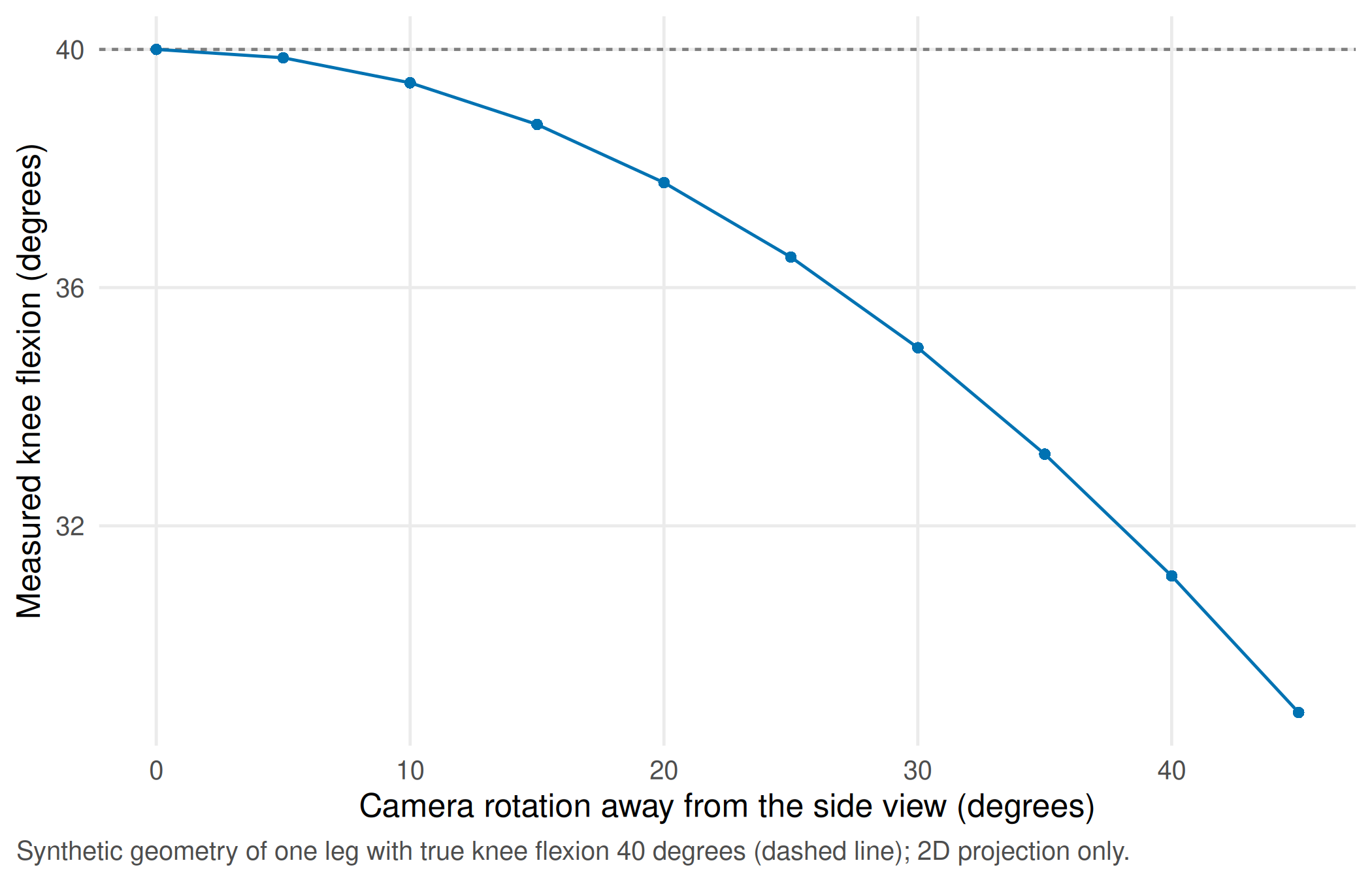
At a camera rotation of 30 degrees, the measured flexion is 35.0 degrees instead of 40: camera position is part of the measurement protocol.
Assumption. For the method comparison, twenty fictitious persons walk five steps each, recorded with both methods from a side view. Before looking at the data, the team fixes a clinical tolerance of ±5 degrees (assumption; a real tolerance needs a clinical justification). Because each person contributes five steps, the steps are averaged per person first: the person is the independent unit.
# Video method against a marker-based reference: 20 fictitious persons, 5 steps each
set.seed(20260416)
persons <- data.frame(person = sprintf("G%02d", 1:20), true_mean = rnorm(20, 60, 5),
                      person_bias = rnorm(20, 0, 1.5))
steps <- persons[rep(1:20, each = 5), ]
steps$step <- rep(1:5, times = 20)
steps$reference <- round(steps$true_mean + rnorm(100, 0, 2), 1)                # degrees
steps$video <- round(steps$reference + 2 + steps$person_bias + rnorm(100, 0, 2.5), 1)
steps <- steps[, c("person", "step", "reference", "video")]
# Aggregate per person first: the person, not the step, is the independent unit
per_person <- aggregate(cbind(reference, video) ~ person, data = steps, FUN = mean)
per_person$mean <- (per_person$reference + per_person$video) / 2
per_person$difference <- per_person$video - per_person$reference
ba <- with(per_person, c(bias = mean(difference), sd = sd(difference)))
loa <- ba[["bias"]] + c(lower = -1.96, upper = 1.96) * ba[["sd"]]
bias_ci_person <- t.test(per_person$difference)$conf.int                       # n = 20 persons
bias_ci_steps  <- t.test(steps$video - steps$reference)$conf.int               # n = 100 steps (pseudoreplication)
tolerance <- 5                                                                 # degrees, assumption set in advance
round(c(ba, loa), 2)
#> bias sd lower upper
#> 1.56 1.90 -2.16 5.28rbind(persons_n20 = bias_ci_person, steps_n100 = bias_ci_steps)#> [,1] [,2]
#> persons_n20 0.6757683 2.452232
#> steps_n100 0.9899886 2.138011stopifnot(nrow(per_person) == 20, length(unique(steps$person)) == 20, nrow(steps) == 100,
diff(bias_ci_steps) < diff(bias_ci_person), # step-level analysis looks falsely precise
loa[["upper"]] > tolerance) # agreement not within the pre-set tolerancep_ba <- ggplot(per_person, aes(mean, difference)) +
annotate("rect", xmin = -Inf, xmax = Inf, ymin = -tolerance, ymax = tolerance, alpha = 0.12,
fill = cdsr_colours[["green"]]) +
geom_hline(yintercept = 0, colour = "grey60") +
geom_hline(yintercept = ba[["bias"]], colour = cdsr_colours[["blue"]]) +
geom_hline(yintercept = loa, colour = cdsr_colours[["blue"]], linetype = "22") +
geom_point(colour = cdsr_colours[["blue"]], shape = cdsr_shapes[1], size = 2.4) +
labs(x = "Mean of video and reference (degrees, mean of 5 steps)",
y = "Video minus reference (degrees)",
caption = "Synthetic data; n = 20 fictitious persons, 5 steps each, averaged per person.\nSolid: bias; dashed: 95% limits of agreement; shaded: tolerance ±5 degrees (assumption).") +
theme_cdsr()
show_figure(p_ba, "w4-bland-altman.png")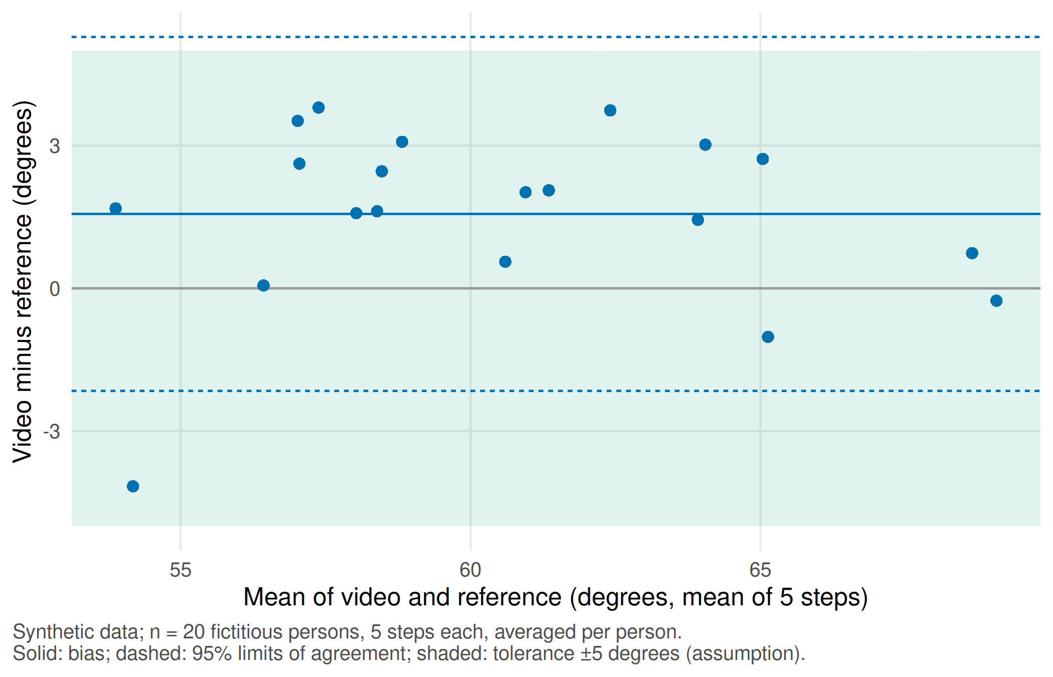
Report. The video method reads on average 1.6 degrees higher than the reference; 95% of per-person differences are expected between -2.2 and 5.3 degrees. The upper limit exceeds the pre-set tolerance of 5 degrees, so the methods should not be used interchangeably for this decision without further work, for example a fixed camera protocol. Note that these limits describe averages of five steps; single steps agree less well.
TipCounter-check: predict first
Would the 95% confidence interval for the bias be wider or narrower if all 100 steps were treated as independent? Compare the two rows printed above: persons (n = 20) give 0.68 to 2.45 degrees, steps (n = 100) give 0.99 to 2.14 degrees. The narrower interval is not more informative; it is falsely precise.
Station tissue: a threshold decides the phenotype
Decision. A spatial-biology group reports that marker-positive cells lie close to blood vessels. The phenotype call “marker-positive” depends on an intensity threshold chosen during image analysis.
Look at the data. Each of six fictitious persons contributes one tissue section of 500 × 500 µm with 250 segmented cells and 15 vessels. Each cell has a marker intensity (0–1) and a distance to the nearest vessel.
Assumption. The threshold of 0.5 is a convention, not a biological fact. We move it to 0.6 and summarise per person, because the person, not the cell, is the independent unit.
# Part C, tissue station (unit 15): synthetic cell positions in one 500 x 500 micrometre field per person
set.seed(20260417)
make_section <- function(person, share_pos) {
  vessels <- data.frame(x = runif(15, 0, 500), y = runif(15, 0, 500))
  n_cells <- 250
  positive <- rbinom(n_cells, 1, share_pos) == 1
  near <- sample(15, n_cells, replace = TRUE)
  x <- ifelse(positive, vessels$x[near] + rnorm(n_cells, 0, 30), runif(n_cells, 0, 500))
  y <- ifelse(positive, vessels$y[near] + rnorm(n_cells, 0, 30), runif(n_cells, 0, 500))
  intensity <- ifelse(positive, rnorm(n_cells, 0.68, 0.12), rnorm(n_cells, 0.38, 0.12))
  cells <- data.frame(person = person, x = pmin(pmax(x, 0), 500), y = pmin(pmax(y, 0), 500),
                      intensity = pmin(pmax(intensity, 0), 1))
  # distance from each cell to the nearest vessel (micrometres)
  cells$dist_vessel <- apply(cells[, c("x", "y")], 1, function(p)
    min(sqrt((vessels$x - p[1])^2 + (vessels$y - p[2])^2)))
  cells
}
cells <- do.call(rbind, Map(make_section, sprintf("S%02d", 1:6), c(0.30, 0.35, 0.40, 0.30, 0.45, 0.50)))
# Phenotype call: marker-positive if the intensity reaches the threshold; compare two thresholds
summarise_threshold <- function(threshold) {
  do.call(rbind, lapply(split(cells, cells$person), function(d) {
    pos <- d$intensity >= threshold
    data.frame(person = d$person[1], threshold = threshold, cells = nrow(d), positive = sum(pos),
               share_positive = mean(pos), median_dist = median(d$dist_vessel[pos]))
  }))
}
tissue <- rbind(summarise_threshold(0.50), summarise_threshold(0.60))
tissue$share_positive <- round(tissue$share_positive, 3)
tissue$median_dist <- round(tissue$median_dist, 1)
rownames(tissue) <- NULL
tissue
#> person threshold cells positive share_positive median_dist
#> 1 S01 0.5 250 90 0.360 39.0
#> 2 S02 0.5 250 108 0.432 41.8
#> 3 S03 0.5 250 116 0.464 32.0
#> 4 S04 0.5 250 92 0.368 38.7
#> 5 S05 0.5 250 125 0.500 30.3
#> 6 S06 0.5 250 126 0.504 31.4
#> 7 S01 0.6 250 57 0.228 34.0
#> 8 S02 0.6 250 73 0.292 37.0
#> 9 S03 0.6 250 78 0.312 30.7
#> 10 S04 0.6 250 60 0.240 34.3
#> 11 S05 0.6 250 88 0.352 27.4
#> 12 S06 0.6 250 93 0.372 28.7low <- tissue[tissue$threshold == 0.50, ]
high <- tissue[tissue$threshold == 0.60, ]
stopifnot(length(unique(cells$person)) == 6, nrow(cells) == 1500,
all(high$share_positive < low$share_positive), # stricter threshold: fewer positive cells
median(high$median_dist) < median(low$median_dist)) # ... which sit closer to vesselstissue_long <- rbind(
data.frame(person = tissue$person, threshold = factor(tissue$threshold),
measure = "Marker-positive cells (%)", value = 100 * tissue$share_positive),
data.frame(person = tissue$person, threshold = factor(tissue$threshold),
measure = "Median distance to vessel (µm)", value = tissue$median_dist))
p_tissue <- ggplot(tissue_long, aes(threshold, value, group = person)) +
geom_line(colour = "grey70") +
geom_point(aes(shape = threshold, colour = threshold), size = 2.4) +
facet_wrap(~ measure, scales = "free_y") +
scale_colour_manual(values = unname(cdsr_colours[c("blue", "orange")])) +
scale_shape_manual(values = cdsr_shapes[1:2]) +
labs(x = "Intensity threshold for 'marker-positive'", y = NULL, colour = "Threshold", shape = "Threshold",
caption = "Synthetic data; n = 6 fictitious persons, one section of 250 cells each; one line per person.") +
theme_cdsr()
show_figure(p_tissue, "w4-tissue.png")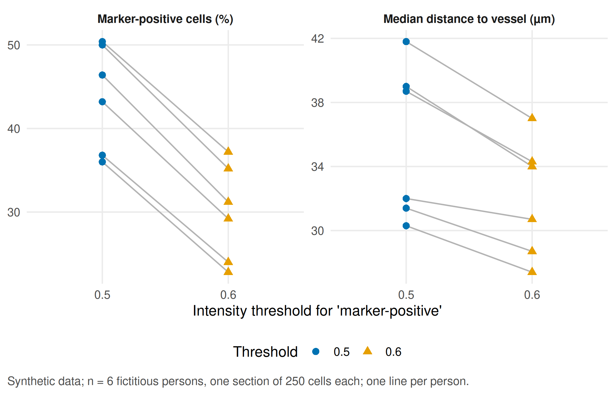
Report. Raising the threshold from 0.5 to 0.6 lowers the share of marker-positive cells in every person (median across persons from 45% to 30%) and makes the remaining positive cells look closer to vessels. The biological conclusion “positive cells cluster near vessels” becomes stronger through an analysis choice. Summarising per person keeps the denominator honest (six persons), but it hides how cells are arranged within each section and how many cells each median rests on; report both.
Your record for the workshop
- The spectral index under the four conditions with the named confounder and the reference measurement you propose (Part A).
- The split table with both target statements, the animal intersection (empty for the animal split) and the independent denominator; one sentence on the limit of generalisation (Part B).
- One figure from your station with unit and independent sample size, and one realistic consequence of the measurement error for a patient or an experiment (Part C).
Download the tables linked at the top if you want to continue in a spreadsheet. The script writes the same files to output/ when you run it on your own.
Further reading
- Companion book: B10 · Hyperspectral imaging and B19 · From one centre or species to the next – required reading for this workshop.
- Companion book: B11 · Measuring gait from video and B12 · Spatial biology and image analysis – background for the two stations.
- Methods in R: Cross-Validation – fold construction and its pitfalls.
- Methods in R: Bland-Altman Limits of Agreement – the agreement analysis behind the gait station.
- Methods in R: ARRIVE — animal research – reporting animal studies, including the experimental unit; see also ARRIVE 2.0.
- CTTIR Courses: Cross-validation, nested CV, bootstrap .632+ – resampling designs in a full lab.
- CTTIR Courses: Kappa, ICC, Bland–Altman – agreement and reliability for measurement comparisons.
- CTTIR Tutorials: Spatial Transcriptomics – spatial data analysis beyond a single threshold.