3  How data arise: missingness and denominators

Author

R. Heller

R. Heller · Date: 2025-04-21 · Last changed: 2026-11-09

NoteAt a glance

Guiding question: Which patient, animal or sample is missing from the table?

For: students and clinical researchers who collect data in routine care or experiments, or receive them as an export · Prerequisites: Chapter 1 (the two teaching datasets and the first R steps)

In the course: W1 · From clinical case to question (required core reading) and W5 · Causality, trajectories and phenotypes · Data: synthetic (generated in the chapter; download b03-visits.csv, b03-patients.csv, b03-dictionary.csv) · Core reading time: about 11 minutes

3.1 Case and decision

The lead physiotherapist of a fictional orthopaedic department prepares a slide for the hospital board. It shows that the mean gait speed of patients after hip fracture surgery rose from 0.33 m/s in the first days to 0.75 m/s three months later. The board is to decide whether the new rehabilitation pathway works and whether to fund two additional therapist posts. The slide is based on an export from the measuring devices. Before it is presented, the department’s data manager asks a simple question: who is in each of these means, and who is not? Of the 12 patients in the cohort, 7 contribute to the three-month value. The others died, were transferred or missed the visit. The decision is how to present the rise: as an effect of rehabilitation, or as a description of the patients who could still be measured.

3.2 Core reading

Core reading · required for W1 · about 11 minutes · ends before ‘Lab’

3.2.1 Every row has a history

Clinical data are a by-product of care. A gait-speed value exists because a test was scheduled, the patient could stand and walk four metres, a therapist had time, the device worked and the export ran. Every missing value also has a reason, and most of these reasons are clinical events: pain, delirium, a transfer, a discharge home, death. An analysis that sees only the exported values sees the end of this process, not the process itself.

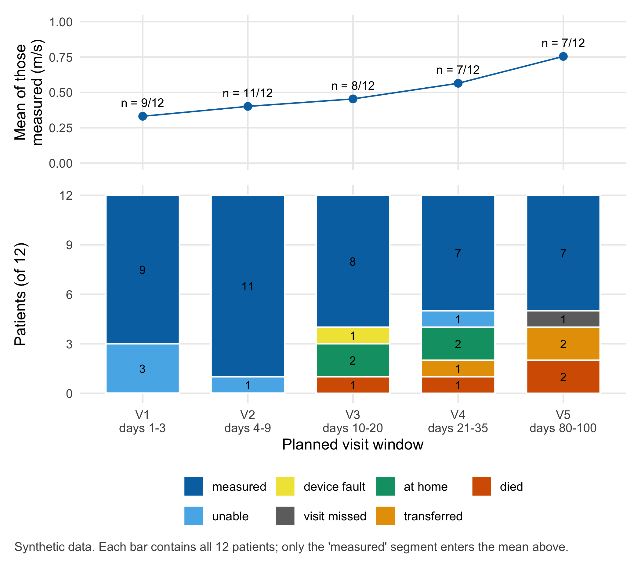
The first tool of this chapter is therefore a planned-visit table: one row for every planned visit of every patient, whether or not a measurement was taken, with a status that says what happened. For the 12 patients of the fracture cohort (Ms K. from Chapter 1 is patient P01) and five planned visit windows, this table has 60 rows. The device export has only 42. Table 3.1 summarises the 60 rows.

Table 3.1: Status of all 60 planned visits in the fracture cohort (n = 12 patients, synthetic). Only the first row contributes to the mean in the last row. Gait speed: 4-metre walk at usual pace, metres per second.
Visit window (days since surgery) V1 (1–3) V2 (4–9) V3 (10–20) V4 (21–35) V5 (80–100)
Measured 9 11 8 7 7
Unable to walk 4 m 3 1 0 1 0
Device fault 0 0 1 0 0
Visit missed 0 0 0 0 1
At home, no visit planned 0 0 2 2 0
Transferred 0 0 0 1 2
Died 0 0 1 1 2
Total patients 12 12 12 12 12
Mean gait speed of those measured (m/s) 0.33 0.40 0.45 0.56 0.75

3.2.2 Different reasons, different consequences

The reasons in Table 3.1 are not interchangeable. Rubin’s classification describes how a missing value relates to the data (Rubin 1976):

  • Missing completely at random (MCAR). The sensor mat failed on day 14 for patient P12. The fault has nothing to do with her walking. Such gaps cost precision but do not distort the mean.
  • Missing at random (MAR). Missingness depends only on information that is already recorded. Patient P03 walked slowly at day 14 (0.38 m/s, recorded) and was transferred to a nursing home; patients P04 and P09 walked fast in the first week (recorded) and went home without inpatient rehabilitation. Because the reason is in the data, methods that use the observed history can, in principle, account for it.
  • Missing not at random (MNAR). “Unable to walk 4 m” means the test was not done because the patient was too slow or unsafe. The missing value depends on itself. No analysis of the observed values alone can repair this without an extra assumption about the values nobody measured.

Two further reasons are not “missing data” in the usual sense. Death ends the existence of a gait speed; there is no value to be missing. The question must say what it means: the gait speed of survivors at day 90, or a combined outcome such as “alive and walking at least 0.6 m/s”. ICH E9(R1) calls death an intercurrent event that must be addressed in the definition of the question itself (International Council for Harmonisation 2019), and Kurland and colleagues show how different analyses answer different questions about data truncated by death (Kurland et al. 2009). Structural gaps arise from the pathway: a patient who went home has no visit in the rehabilitation clinic because none was planned.

The consequence for the board slide is uncomfortable. In windows V3 and V4 the two fastest patients of the first week are missing (they went home), together with some of the slowest. In V5 mainly the slowest are missing (they died or were transferred). The rise from 0.56 to 0.75 m/s between V4 and V5 is partly a change in who is measured. Every mean in a longitudinal table is a mean of those measured at that time; without the planned-visit table nobody can tell whether a change over time is a change in patients or a change in who is counted. The Lab draws this as a figure with the denominator written above every point.

3.2.3 Many rows, few units

The second trap is the opposite of a missing row: too many rows. In the HSI rat study of Chapter 1, each of six animals contributes two limbs, two images per limb and 200 pixels per image: 4,800 rows. Treating the pixels as independent observations is pseudoreplication, defined by Hurlbert as testing a treatment effect with replicates that are not statistically independent (Hurlbert 1984). In a survey of one issue of a neuroscience journal, Lazic found pseudoreplication in 12% of papers and suspected it in a further 36% (published) (Lazic 2010). In the Lab, the pixel analysis of our synthetic rats gives an interval of −5.1 to −4.1 percentage points for the difference in oxygenation between injured and control limb. Analysed per animal, the interval is −11.3 to +2.1: the data are compatible with no difference at all. The same applies to the fracture cohort: 42 gait-speed values come from 11 patients, not from 42. ARRIVE 2.0 therefore asks every animal study to name its experimental unit (Percie du Sert et al. 2020).

3.2.4 Rare combinations identify people

The third question concerns a teaching dataset leaving the hospital. Individual attributes such as age, sex, injury, accident mechanism, admission date or postal district look harmless. Their combination is not. In a synthetic registry extract of 403 patients built in the Lab, every record is unique on these six attributes. One record describes a 34-year-old woman admitted on 14 August after a paragliding accident with a scapulothoracic dissociation, a rare injury. The injury alone is unique; a short local news report would be enough to name her. Rocher and colleagues estimated that 99.98% of Americans would be correctly re-identified in any dataset using 15 demographic attributes (published) (Rocher et al. 2019). Sweeney’s k-anonymity formalises the defence: each released record should be indistinguishable from at least k − 1 others on the attributes an outsider could know (Sweeney 2002). For teaching, the remedy is mostly subtraction: keep only the columns the exercise needs, coarsen the rest, and leave out what remains unique.

Question for the workshop: Rewrite the board slide. Under each of the five points, write the denominator and the reason why patients are missing. Which point would you remove or label differently, and why?

3.3 Lab

3.3.1 Step 1: the patient table and the planned-visit table

The data come in two tables, as they would in a real project. patients has one row per patient; visits has one row per planned visit. The column pid links them. rbind() stacks the rows of several small tables; NA is R’s code for “not available”.

patients <- data.frame(
  pid        = sprintf("P%02d", 1:12),
  age        = c(84, 79, 91, 76, 93, 82, 80, 88, 74, 86, 90, 78),       # years at admission
  sex        = c("f", "f", "f", "m", "f", "f", "m", "f", "f", "m", "f", "f"),
  fracture   = c("neck", "pertroch", "pertroch", "neck", "pertroch", "neck",
                 "neck", "pertroch", "neck", "pertroch", "neck", "neck"),
  end_day    = c(91, 88, 20, 90, 11, 90, 93, 33, 90, 90, 52, 89),       # days since surgery
  end_reason = c("follow-up complete", "follow-up complete", "transferred to nursing home",
                 "follow-up complete", "died", "day-90 visit missed", "follow-up complete",
                 "transferred to acute hospital", "follow-up complete", "follow-up complete",
                 "died", "follow-up complete")
)

windows <- c("V1", "V2", "V3", "V4", "V5")
visit_rows <- function(pid, day, gait_ms, status) {          # five planned visits of one patient
  data.frame(pid = pid, window = windows, day = day, gait_ms = gait_ms, status = status)
}
m <- "measured"
visits <- rbind(
  visit_rows("P01", c(2, 6, 15, 27, 91), c(.31, .42, .55, .63, .78), rep(m, 5)),
  visit_rows("P02", c(1, 5, 13, 29, 88), c(.28, .35, .47, .58, .70), rep(m, 5)),
  visit_rows("P03", c(2, 6, 14, NA, NA), c(NA, .31, .38, NA, NA),
             c("unable", m, m, "transferred", "transferred")),
  visit_rows("P04", c(3, 8, NA, NA, 90), c(.40, .52, NA, NA, .85),
             c(m, m, "at home", "at home", m)),
  visit_rows("P05", c(1, 4, NA, NA, NA), c(NA, NA, NA, NA, NA),
             c("unable", "unable", "died", "died", "died")),
  visit_rows("P06", c(2, 7, 16, 30, NA), c(.33, .41, .50, .57, NA),
             c(m, m, m, m, "visit missed")),
  visit_rows("P07", c(2, 6, 12, 26, 93), c(.36, .47, .58, .66, .81), rep(m, 5)),
  visit_rows("P08", c(3, 8, 17, 31, NA), c(NA, .30, .29, NA, NA),
             c("unable", m, m, "unable", "transferred")),
  visit_rows("P09", c(2, 5, NA, NA, 90), c(.38, .49, NA, NA, .88),
             c(m, m, "at home", "at home", m)),
  visit_rows("P10", c(2, 9, 18, 28, 90), c(.27, .33, .41, .46, .52), rep(m, 5)),
  visit_rows("P11", c(1, 6, 15, 24, NA), c(.30, .37, .45, .44, NA), c(m, m, m, m, "died")),
  visit_rows("P12", c(3, 7, 14, 28, 89), c(.35, .44, NA, .61, .74),
             c(m, m, "device fault", m, m))
)
visits$method <- ifelse(visits$window %in% c("V3", "V4"), "sensor mat", "stopwatch")
visits$method[is.na(visits$day)] <- NA     # no visit took place, so no method
head(visits, 7)
#>   pid window day gait_ms   status     method
#> 1 P01     V1   2    0.31 measured  stopwatch
#> 2 P01     V2   6    0.42 measured  stopwatch
#> 3 P01     V3  15    0.55 measured sensor mat
#> 4 P01     V4  27    0.63 measured sensor mat
#> 5 P01     V5  91    0.78 measured  stopwatch
#> 6 P02     V1   1    0.28 measured  stopwatch
#> 7 P02     V2   5    0.35 measured  stopwatch

The first seven rows show patient P01 completely and the start of P02. Each row answers four questions: who (pid), which planned visit (window), when it actually happened (day, days since surgery) and what came out (gait_ms and status). This layout, one row per observation and one column per variable, is called long or tidy; Chapter 4 explains why it is the right format for analysis.

3.3.2 Step 2: the data dictionary

A table without a description is a puzzle for the next person. A data dictionary names, for each column, its meaning, type, unit, time reference and the plausible reasons for a missing value (Broman and Woo 2018).

dictionary <- data.frame(
  table    = c(rep("patients", 6), rep("visits", 6)),
  variable = c("pid", "age", "sex", "fracture", "end_day", "end_reason",
               "pid", "window", "day", "gait_ms", "status", "method"),
  meaning  = c("Pseudonymous patient identifier (P01-P12); key", "Age at admission",
               "Sex as recorded (f, m)", "Fracture type: femoral neck (neck) or pertrochanteric (pertroch)",
               "Last day of follow-up", "Why follow-up ended",
               "Link to the patients table", "Planned window: V1 1-3, V2 4-9, V3 10-20, V4 21-35, V5 80-100",
               "Actual day of the visit", "Gait speed, 4-metre walk at usual pace",
               "measured, unable, device fault, visit missed, at home, transferred, died",
               "stopwatch (ward, outpatient) or sensor mat (rehabilitation)"),
  type     = c("text", "number", "text", "text", "number", "text",
               "text", "text", "number", "number", "text", "text"),
  unit     = c("-", "years", "-", "-", "days since surgery", "-",
               "-", "days since surgery", "days since surgery", "m/s", "-", "-"),
  missing_when = c("never", "never", "never", "never", "never", "never",
                   "never", "never", "no visit took place", "status is not 'measured'",
                   "never", "no visit took place")
)
knitr::kable(dictionary)
Table 3.2: Data dictionary of the fracture cohort (synthetic). Time zero for all day counts is the day of surgery (day 0).
table variable meaning type unit missing_when
patients pid Pseudonymous patient identifier (P01-P12); key text - never
patients age Age at admission number years never
patients sex Sex as recorded (f, m) text - never
patients fracture Fracture type: femoral neck (neck) or pertrochanteric (pertroch) text - never
patients end_day Last day of follow-up number days since surgery never
patients end_reason Why follow-up ended text - never
visits pid Link to the patients table text - never
visits window Planned window: V1 1-3, V2 4-9, V3 10-20, V4 21-35, V5 80-100 text days since surgery never
visits day Actual day of the visit number days since surgery no visit took place
visits gait_ms Gait speed, 4-metre walk at usual pace number m/s status is not ‘measured’
visits status measured, unable, device fault, visit missed, at home, transferred, died text - never
visits method stopwatch (ward, outpatient) or sensor mat (rehabilitation) text - no visit took place

Two entries deserve a comment. The method changes from stopwatch to sensor mat between V2 and V3, because the rehabilitation clinic uses a different device. A jump in the curve at that point may be a measurement artefact; how large the systematic difference between the two methods is remains open in this cohort (Chapter 11 treats method comparison). And status is never missing: it is the column that makes every gap explainable.

3.3.3 Step 3: counts and denominators

table() counts combinations; tapply() applies a function, here the mean, within groups. na.rm = TRUE tells mean() to ignore missing values, which is exactly the step that hides the denominator.

status_levels <- c("measured", "unable", "device fault", "visit missed", "at home", "transferred", "died")
visits$status <- factor(visits$status, levels = status_levels)
status_table <- table(visits$status, visits$window)
status_table
#>               
#>                V1 V2 V3 V4 V5
#>   measured      9 11  8  7  7
#>   unable        3  1  0  1  0
#>   device fault  0  0  1  0  0
#>   visit missed  0  0  0  0  1
#>   at home       0  0  2  2  0
#>   transferred   0  0  0  1  2
#>   died          0  0  1  1  2
mean_by_window <- tapply(visits$gait_ms, visits$window, mean, na.rm = TRUE)
round(mean_by_window, 2)
#>   V1   V2   V3   V4   V5 
#> 0.33 0.40 0.45 0.56 0.75
stopifnot(
  all(colSums(status_table) == 12),                                   # every window holds all 12 patients
  status_table["measured", ] == c(9, 11, 8, 7, 7),                    # as in the Core reading table
  round(mean_by_window, 2) == c(0.33, 0.40, 0.45, 0.56, 0.75)
)

3.3.4 Step 4: patients, measurements and linked records, counted twice

Counting looks trivial, and that is why errors survive. Below, each number is computed on two independent paths: path A from the visit table, path B from other objects or with other functions. The numbers are accepted only if both paths agree.

# path A: from the visit table
a <- c(patients      = length(unique(visits$pid)),
       measurements  = sum(visits$status == "measured"),
       with_value    = length(unique(visits$pid[!is.na(visits$gait_ms)])),
       linked        = nrow(merge(visits[!is.na(visits$gait_ms), ], patients, by = "pid")))
# path B: from the patient table, per-patient sums and a matching test
per_patient <- tapply(!is.na(visits$gait_ms), visits$pid, sum)
b <- c(patients      = nrow(patients),
       measurements  = sum(per_patient),
       with_value    = sum(per_patient > 0),
       linked        = sum(visits$pid[!is.na(visits$gait_ms)] %in% patients$pid))
rbind(path_A = a, path_B = b)
#>        patients measurements with_value linked
#> path_A       12           42         11     42
#> path_B       12           42         11     42
stopifnot(identical(a, b), b[["patients"]] == 12, b[["measurements"]] == 42,
          b[["with_value"]] == 11, b[["linked"]] == 42)
names(per_patient)[per_patient == 0]     # the patient who never appears in the device export
#> [1] "P05"

Twelve patients, 42 measurements, all 42 linked to a patient, but only 11 patients with any value. Patient P05 was unable to walk at both early visits and died on day 11. She exists in the patient table and in the planned-visit table, but not in any device export: precisely the person the board slide does not show.

3.3.5 Step 5: first trajectory figure, individual courses

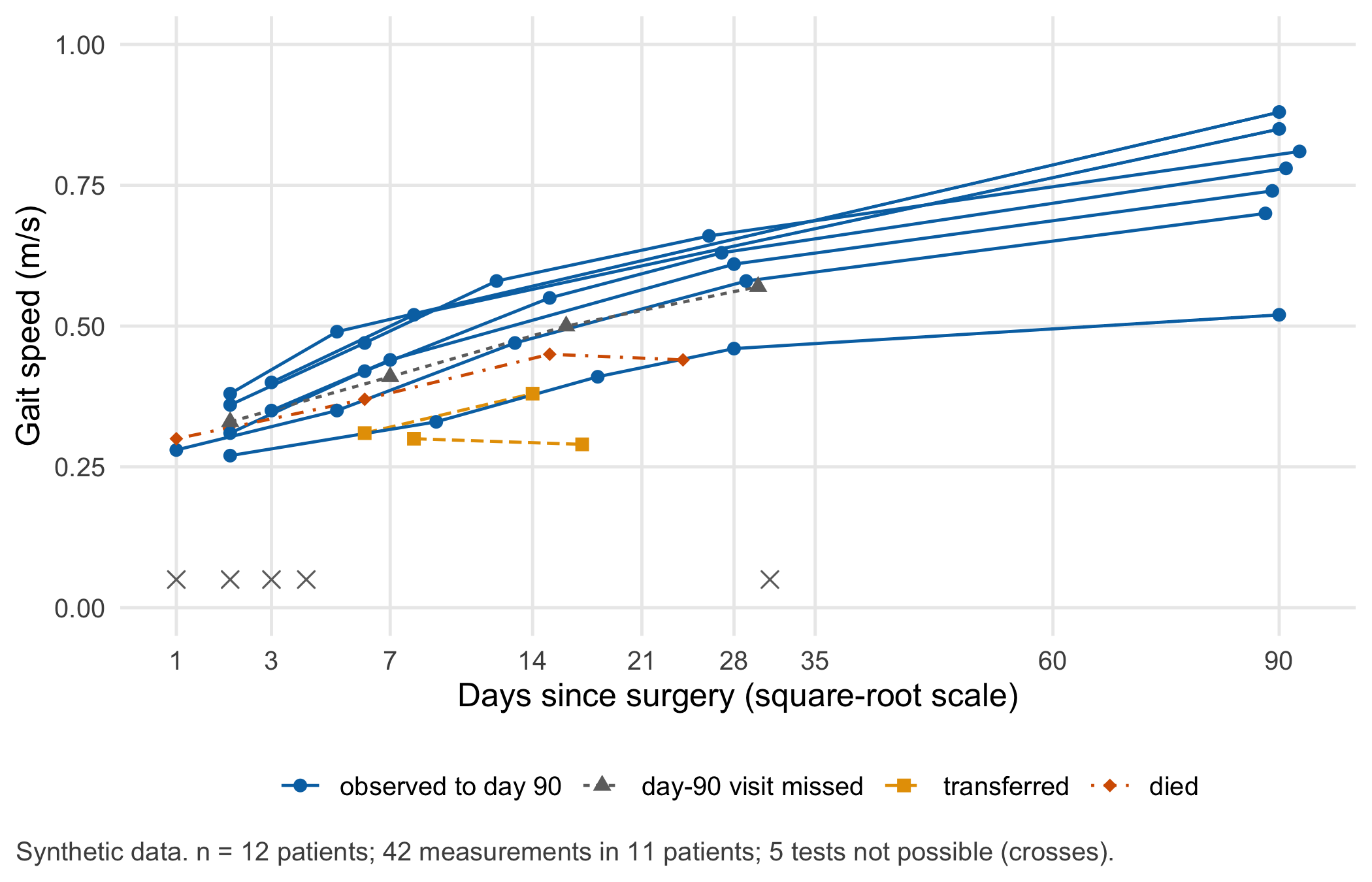
A spaghetti plot draws one line per patient. Colour, line type and point shape show how follow-up ended; crosses at the bottom mark visits where the test was attempted but not possible.

library(ggplot2)
course_of <- c("follow-up complete" = "observed to day 90", "day-90 visit missed" = "day-90 visit missed",
               "transferred to nursing home" = "transferred", "transferred to acute hospital" = "transferred",
               "died" = "died")
measured <- merge(visits[visits$status == "measured", ], patients[, c("pid", "end_reason")], by = "pid")
measured$course <- factor(course_of[measured$end_reason],
                          levels = c("observed to day 90", "day-90 visit missed", "transferred", "died"))
unable <- visits[visits$status == "unable", ]

ggplot(measured, aes(x = day, y = gait_ms, group = pid, colour = course, linetype = course, shape = course)) +
  geom_line() +
  geom_point(size = 2) +
  geom_point(data = unable, aes(x = day, y = 0.05), inherit.aes = FALSE,
             shape = 4, size = 2.5, colour = cdsr_colours[["grey"]]) +
  scale_x_continuous(transform = "sqrt", breaks = c(1, 3, 7, 14, 21, 28, 35, 60, 90)) +
  scale_y_continuous(limits = c(0, 1)) +
  scale_colour_manual(values = unname(cdsr_colours[c("blue", "grey", "orange", "red")])) +
  scale_linetype_manual(values = cdsr_linetypes) +
  scale_shape_manual(values = cdsr_shapes) +
  labs(x = "Days since surgery (square-root scale)", y = "Gait speed (m/s)",
       colour = NULL, linetype = NULL, shape = NULL,
       caption = "Synthetic data. n = 12 patients; 42 measurements in 11 patients; 5 tests not possible (crosses).") +
  theme_cdsr()
Line chart of gait speed against days since surgery for eleven patients. Most lines rise from about 0.3 metres per second in the first days to between 0.5 and 0.9 metres per second at day 90. Two transferred patients stop at days 14 and 17 below 0.4, one patient who died stops at day 24, and one patient who missed the last visit stops at day 30. The twelfth patient, who died on day 11, has no line because she was never able to walk 4 metres. Five crosses near the bottom mark tests that were not possible, four in the first week and one at day 31.
Figure 3.1: Gait speed (m/s) after hip fracture surgery, one line per patient, by how follow-up ended. Crosses at 0.05 m/s: test attempted but patient unable to walk 4 m. Horizontal axis on a square-root scale. n = 12 patients; 42 measurements from 11 patients; synthetic.

3.3.6 Step 6: second trajectory figure, means with their denominators

The second figure shows what the board slide showed, the mean per window, but writes the denominator above every point and shows, underneath, what happened to all 12 patients in that window. ggplot2 draws the two panels; patchwork stacks them.

library(patchwork)
summary_win <- data.frame(window = names(mean_by_window),
                          mean_ms = as.vector(mean_by_window),
                          n = as.vector(status_table["measured", ]))
window_labels <- c(V1 = "V1\ndays 1-3", V2 = "V2\ndays 4-9", V3 = "V3\ndays 10-20",
                   V4 = "V4\ndays 21-35", V5 = "V5\ndays 80-100")

top <- ggplot(summary_win, aes(x = window, y = mean_ms, group = 1)) +
  geom_line(colour = cdsr_colours[["blue"]]) +
  geom_point(colour = cdsr_colours[["blue"]], size = 2.5) +
  geom_text(aes(label = paste0("n = ", n, "/12")), vjust = -1.1, size = 3.3) +
  scale_y_continuous(limits = c(0, 1)) +
  scale_x_discrete(labels = NULL) +
  labs(x = NULL, y = "Mean of those\nmeasured (m/s)") +
  theme_cdsr()

counts <- as.data.frame(status_table, responseName = "patients")
names(counts)[1:2] <- c("status", "window")
bottom <- ggplot(counts, aes(x = window, y = patients, fill = status)) +
  geom_col(width = 0.7, colour = "white") +
  geom_text(aes(label = ifelse(patients > 0, patients, "")),
            position = position_stack(vjust = 0.5), size = 3.2) +
  scale_fill_manual(values = unname(cdsr_colours[c("blue", "skyblue", "yellow", "grey", "green", "orange", "red")])) +
  scale_x_discrete(labels = window_labels) +
  scale_y_continuous(breaks = c(0, 3, 6, 9, 12)) +
  labs(x = "Planned visit window", y = "Patients (of 12)", fill = NULL,
       caption = "Synthetic data. Each bar contains all 12 patients; only the 'measured' segment enters the mean above.") +
  theme_cdsr() +
  guides(fill = guide_legend(nrow = 2))

top / bottom + plot_layout(heights = c(1, 1.4))
Two stacked panels. The upper panel is a line through five points rising from 0.33 metres per second in window V1 to 0.75 in window V5, labelled n equals 9, 11, 8, 7 and 7 of 12. The lower panel shows five stacked bars of height 12. Measured patients form the largest segment in each bar. In V1 three patients were unable to walk; in V3 and V4 two patients were at home; in V5 two had died, two were transferred and one visit was missed.
Figure 3.2: Top: mean gait speed (m/s) of the patients measured in each planned visit window, with the observed denominator. Bottom: status of all 12 patients in each window (number of patients written in each segment). n = 12 patients, 60 planned visits; synthetic.

The upper panel alone is the board slide. With the lower panel, the reader sees that the five means describe five different groups of patients.

3.3.7 Step 7: saving the tables for the next chapter

The three tables are written as plain-text CSV files into the book’s data folder, using a path relative to this chapter (.. means “one folder up”). Chapter 4 rebuilds them from raw exports and checks that it gets exactly these files.

visits_out <- visits
visits_out$status <- as.character(visits_out$status)    # store plain text, not R factor codes
write.csv(patients,   "../data/b03-patients.csv",   row.names = FALSE)
write.csv(visits_out, "../data/b03-visits.csv",     row.names = FALSE)
write.csv(dictionary, "../data/b03-dictionary.csv", row.names = FALSE)
stopifnot(nrow(read.csv("../data/b03-visits.csv")) == 60)

3.3.8 Step 8: pseudoreplication in the HSI rat study

The rat data are generated by a function with its own seed. Oxygen saturation (StO2) is given in percent; each animal has its own baseline and its own injury effect, and each image adds a small shift.

make_hsi <- function(seed = 7) {
  set.seed(seed)
  animal_diff <- rnorm(6, mean = -3, sd = 5)       # injured minus control, percentage points (assumption)
  animal_base <- rnorm(6, mean = 70, sd = 4)       # StO2 of the control limb, percent (assumption)
  grid <- expand.grid(pixel = 1:200, image = 1:2, limb = c("control", "injured"),
                      animal = sprintf("A%d", 1:6), stringsAsFactors = FALSE)
  i <- match(grid$animal, sprintf("A%d", 1:6))
  image_shift <- rnorm(24, 0, 1.5)[as.integer(factor(paste(grid$animal, grid$limb, grid$image)))]
  mu <- animal_base[i] + (grid$limb == "injured") * animal_diff[i] + image_shift
  grid$sto2 <- round(rnorm(nrow(grid), mu, 6), 1)  # pixel noise
  grid[, c("animal", "limb", "image", "pixel", "sto2")]
}
hsi <- make_hsi()
c(rows = nrow(hsi), animals = length(unique(hsi$animal)))
#>    rows animals 
#>    4800       6
# wrong unit: every pixel treated as an independent observation
pixel_ci <- t.test(hsi$sto2[hsi$limb == "injured"], hsi$sto2[hsi$limb == "control"])$conf.int
# right unit: one difference per animal (injured minus control), six values
animal_means <- tapply(hsi$sto2, list(hsi$animal, hsi$limb), mean)
animal_diff  <- animal_means[, "injured"] - animal_means[, "control"]
animal_ci <- t.test(animal_diff)$conf.int
round(rbind(pixels_as_units = pixel_ci, animals_as_units = animal_ci), 1)
#>                   [,1] [,2]
#> pixels_as_units   -5.1 -4.1
#> animals_as_units -11.3  2.1
stopifnot(pixel_ci[2] < 0, animal_ci[1] < 0, animal_ci[2] > 0,
          round(c(pixel_ci, animal_ci), 1) == c(-5.1, -4.1, -11.3, 2.1))

Both intervals are centred near the same difference (about -4.6 percentage points), but the pixel interval is about 13 times narrower and excludes zero, while the animal interval includes it. The pixel analysis answers a question nobody asked: how precisely the 4,800 pixel values of these six rats are known. The research question concerns rats in general, and its sample size is six. Mixed models that keep the pixel level are introduced in Chapter 13; Chapter 10 and Chapter 19 build on this with spectra and splits by animal.

3.3.9 Step 9: rare combinations in a registry extract

The last step builds a synthetic registry extract of 400 common fractures and adds three rare, severe injuries. The function k_size() returns, for each record, how many records share its values on the chosen columns: the k of k-anonymity. A record with k = 1 is unique.

make_registry <- function(seed = 3107, n = 400) {
  set.seed(seed)
  injury <- sample(c("distal radius fracture", "proximal femur fracture", "ankle fracture",
                     "proximal humerus fracture", "vertebral fracture"), n, replace = TRUE,
                   prob = c(0.30, 0.25, 0.20, 0.15, 0.10))
  age_mean <- c("distal radius fracture" = 62, "proximal femur fracture" = 83, "ankle fracture" = 50,
                "proximal humerus fracture" = 72, "vertebral fracture" = 68)[injury]
  age <- pmin(99, pmax(18, round(rnorm(n, age_mean, 12))))
  sex <- ifelse(runif(n) < ifelse(injury == "ankle fracture", 0.5, 0.7), "f", "m")
  mechanism <- ifelse(age >= 70, "fall from standing height",
                      sample(c("fall from standing height", "road traffic", "sport", "fall from height"),
                             n, replace = TRUE, prob = c(0.40, 0.25, 0.25, 0.10)))
  admission <- as.Date("2025-01-01") + sample(0:364, n, replace = TRUE)
  district <- sample(c("890", "891", "892", "893", "894", "895"), n, replace = TRUE)
  common <- data.frame(rid = sprintf("R%03d", 1:n), age, sex, injury, mechanism, admission, district)
  rare <- data.frame(rid = c("R401", "R402", "R403"), age = c(34, 41, 57), sex = c("f", "m", "m"),
                     injury = c("scapulothoracic dissociation", "open pelvic fracture", "open pelvic fracture"),
                     mechanism = c("paragliding", "road traffic", "fall from height"),
                     admission = as.Date(c("2025-08-14", "2025-03-02", "2025-11-20")),
                     district = c("893", "890", "895"))
  rbind(common, rare)
}
k_size <- function(data, columns) {
  key <- do.call(paste, c(data[columns], sep = "|"))
  as.vector(table(key)[key])
}
registry <- make_registry()
all_six <- c("age", "sex", "injury", "mechanism", "admission", "district")
c(records = nrow(registry), unique_on_all_six = sum(k_size(registry, all_six) == 1))
#>           records unique_on_all_six 
#>               403               403

Every one of the 403 records is unique on the six attributes. The table below shows how many records share their values with record R401, the paragliding accident, when only some attributes are released.

registry$admission_month <- format(registry$admission, "%m")
registry$age_band  <- cut(registry$age, c(17, 49, 69, 84, 120), labels = c("18-49", "50-69", "70-84", "85+"))
registry$injury_group <- ifelse(registry$injury %in% c("scapulothoracic dissociation", "open pelvic fracture"),
                                "other severe injury", registry$injury)
released <- list("injury"                           = "injury",
                 "sex + mechanism"                  = c("sex", "mechanism"),
                 "age + sex"                        = c("age", "sex"),
                 "sex + district + admission month" = c("sex", "district", "admission_month"),
                 "age band + sex + injury group"    = c("age_band", "sex", "injury_group"))
k_r401 <- sapply(released, function(cols) k_size(registry, cols)[registry$rid == "R401"])
k_r401
#>                           injury                  sex + mechanism 
#>                                1                                1 
#>                        age + sex sex + district + admission month 
#>                                2                                4 
#>    age band + sex + injury group 
#>                                1
stopifnot(k_r401 == c(1, 1, 2, 4, 1))

Even after grouping the rare injuries and banding the age, R401 remains unique, because she is the only woman under 50 with a severe injury other than a common fracture. The teaching purpose decides what can go. Suppose the exercise is to compare length of stay between injury groups in younger and older patients. Then sex, mechanism, date and district are not needed at all (data minimisation), age needs only two bands, and records that remain rare are left out of the teaching file.

registry$age_2 <- ifelse(registry$age < 70, "18-69", "70+")
k_teaching <- k_size(registry, c("age_2", "injury_group"))
teaching <- registry[k_teaching >= 5, c("rid", "age_2", "injury_group")]
c(records_kept = nrow(teaching), records_left_out = sum(k_teaching < 5),
  smallest_k_after = min(k_size(teaching, c("age_2", "injury_group"))))
#>     records_kept records_left_out smallest_k_after 
#>              400                3                5
stopifnot(sum(k_teaching < 5) == 3, min(k_size(teaching, c("age_2", "injury_group"))) >= 5,
          !"R401" %in% teaching$rid)

The reduced teaching file keeps 400 of 403 records on two columns, and every record shares its values with at least four others. The three severe rare injuries are left out; the file says so in its documentation, because their absence is itself a missing-data mechanism for anyone studying severe trauma with it. Whether such a reduced extract would be anonymous in the legal sense is a separate question (see below).

3.4 Counter-check

Because the cohort is synthetic, we know the gait speeds that could not be measured: the values the simulation assumed for the five “unable” visits. Real data never offer this. Predict first: if these patients had been measured, would the means in V1, V2 and V4 rise or fall, and in which window would the change be largest?

hidden <- data.frame(pid    = c("P03", "P05", "P05", "P08", "P08"),
                     window = c("V1", "V1", "V2", "V1", "V4"),
                     gait_ms_hidden = c(0.15, 0.12, 0.16, 0.17, 0.21))   # known only in the simulation
completed <- merge(visits, hidden, by = c("pid", "window"), all.x = TRUE)
completed$gait_ms_all <- ifelse(is.na(completed$gait_ms), completed$gait_ms_hidden, completed$gait_ms)
mean_if_tested <- tapply(completed$gait_ms_all, completed$window, mean, na.rm = TRUE)
round(rbind(observed = mean_by_window, if_unable_were_tested = mean_if_tested), 3)
#>                          V1    V2    V3    V4    V5
#> observed              0.331 0.401 0.454 0.564 0.754
#> if_unable_were_tested 0.285 0.381 0.454 0.520 0.754
stopifnot(all(mean_if_tested[c("V1", "V2", "V4")] < mean_by_window[c("V1", "V2", "V4")]),
          which.max(mean_by_window - mean_if_tested) == 1)

All three means fall, most in V1 (by 0.046 m/s), where three of twelve patients could not be tested. The rise across the whole follow-up becomes steeper, not flatter, because the early values were too optimistic. Nothing comparable is possible for V5: the two patients who died have no gait speed at day 90, so the question itself must be redefined (survivors only, or a combined outcome), not the data completed.

3.5 Consequences for patients and operations

Patients. Means of “those measured” systematically leave out the frailest: those unable to walk, transferred or dead. A board slide that hides them can lead to funding decisions that look successful because the patients who fared worst have vanished from the graph. Showing denominators is a matter of fairness to those patients, not only of statistics.

Operations. The planned-visit table needs a status column that clinical staff fill in at the time, with a short list of allowed values. Adding the reasons months later from memory turns MNAR into guesswork. A change of measuring device must be recorded in the data, with its date. Reports should show per-window denominators by default.

Data protection. Gait speed is data concerning health, a special category under Article 9(1) of the General Data Protection Regulation (GDPR, Regulation (EU) 2016/679) (European Parliament and Council of the European Union 2016), published on 4 May 2016, in force since 24 May 2016 and applicable since 25 May 2018. Replacing names by identifiers such as P01 is pseudonymisation in the sense of Article 4(5); Recital 26 states that pseudonymised data which could be attributed to a person by additional information remain information on an identifiable person, while anonymous information falls outside the Regulation. Article 5(1)(c) requires data to be limited to what is necessary (data minimisation), and Article 89(1) requires safeguards for research, including that research purposes which can be fulfilled without identifying data subjects shall be fulfilled in that manner (status: November 2026). Whether a reduced extract like the one in Step 9 is anonymous depends on all means reasonably likely to be used for identification, including local news reports and other registries. That assessment is open for any real dataset and belongs to the data protection officer of the institution, not to the analyst (Chapter 23, Chapter 26).

Animal research. Reporting 4,800 pixels as the sample size would overstate the evidence from six animals and could justify further experiments on a false basis. ARRIVE 2.0 asks for the experimental unit to be stated for each experiment (item 1b); see also Chapter 16 for small samples and the 3Rs.

3.6 Look up and transfer

  • Reviewer question: For every mean or proportion reported over time: what is the denominator at that time, who is missing, and for which documented reason?

  • Self-test: On an intensive care unit, C-reactive protein (CRP) is measured daily in unstable patients and twice a week in stable ones. A study reports the mean of all CRP values per patient-week and finds that “CRP is higher in the first week”. What is the problem with the denominator, and how would you analyse it instead?

    The number of measurements depends on how ill a patient is: unstable patients contribute more values, so a mean over all measurements is weighted towards the sickest patients and towards the days on which they were sickest. The visit process is informative. Summarise per patient first (for example one mean or the last value per patient and week), report how many patients contribute to each week, and treat patients who died or were discharged as an explicit status, not as missing values.

  • Annotated sources:

    • Rubin (1976) — the original definitions behind MCAR, MAR and MNAR.
    • International Council for Harmonisation (2019) — death and transfer as intercurrent events that belong in the question.
    • Kurland et al. (2009) — which analysis answers which question when follow-up is truncated by death.
    • Hurlbert (1984) — the definition of pseudoreplication.
    • Lazic (2010) — how often pseudoreplication occurs in laboratory research (published figures).
    • Sweeney (2002) — k-anonymity as a criterion for released records.
    • Rocher et al. (2019) — how few attributes suffice to re-identify people (published estimate).
    • Broman and Woo (2018) — practical rules for tables and data dictionaries.
    • European Parliament and Council of the European Union (2016) — GDPR Articles 4(5), 5(1)(c), 9(1) and 89(1), and Recital 26, as cited above.

3.7 Further reading