library(ggplot2)
library(glmnet)Lab W3 · Two-by-two tables, baseline and threshold
Teaching units 09–11: predictive values at two prevalences, a logistic baseline against a tuned alternative, calibration, threshold and errors by subgroup.
Every part of this lab follows the same five steps: state the decision, look at the data, name the assumption, compute in R and write one sentence for the person who has to act. All numbers are synthetic or teaching assumptions; none describes a commercial product or a real emergency department.
If R is new to you, read the code and the printed output first and answer the questions on paper; the printed results are complete. If you are fluent in R, try the extra counter-check at the end of each part.
Part A · The same alert in two referral settings (unit 09)
Decision. A fictitious emergency department considers a tool that suggests a second look at a wrist radiograph when it flags a possible fracture. Clinicians want to know how many alerts per shift will turn out to be fractures.
Assumption. In both settings the tool has a sensitivity and a specificity of 90% (assumption). In the first setting 5 of 100 people examined have a fracture, in the second 20 of 100. Whether the tool really reaches 90% in either setting is open and would need a local study.
Before you run the code, cover the right-hand columns of the printed table and fill in a two-by-two table for 1,000 examinations by hand. Who belongs in the denominator of the positive predictive value?
# Part A (unit 09): 1,000 examinations in each of two referral settings
scenarios <- data.frame(
  setting     = c("Low prevalence (5%)", "Higher prevalence (20%)"),
  n           = c(1000, 1000),
  prevalence  = c(0.05, 0.20),
  sensitivity = c(0.90, 0.90),   # assumption, identical in both settings
  specificity = c(0.90, 0.90)    # assumption, identical in both settings
)
scenarios$fracture    <- scenarios$n * scenarios$prevalence
scenarios$no_fracture <- scenarios$n - scenarios$fracture
scenarios$tp <- scenarios$sensitivity * scenarios$fracture       # true alerts
scenarios$fn <- scenarios$fracture - scenarios$tp                # missed fractures
scenarios$tn <- scenarios$specificity * scenarios$no_fracture    # correct all-clear
scenarios$fp <- scenarios$no_fracture - scenarios$tn             # false alerts
scenarios$alerts <- scenarios$tp + scenarios$fp
scenarios$ppv <- scenarios$tp / scenarios$alerts                 # share of alerts that are fractures
scenarios$npv <- scenarios$tn / (scenarios$tn + scenarios$fn)    # share of all-clears without fracture
print(scenarios[, c("setting", "tp", "fp", "fn", "tn", "alerts", "ppv", "npv")], digits = 3)
#> setting tp fp fn tn alerts ppv npv
#> 1 Low prevalence (5%) 45 95 5 855 140 0.321 0.994
#> 2 Higher prevalence (20%) 180 80 20 720 260 0.692 0.973# Target values of the teaching case: TP/FP/FN/TN = 45/95/5/855 and 180/80/20/720
stopifnot(
isTRUE(all.equal(scenarios$tp, c(45, 180))),
isTRUE(all.equal(scenarios$fp, c(95, 80))),
isTRUE(all.equal(scenarios$fn, c(5, 20))),
isTRUE(all.equal(scenarios$tn, c(855, 720))),
isTRUE(all.equal(scenarios$alerts, c(140, 260))),
identical(cdsr_percent(scenarios$ppv), c("32.1%", "69.2%"))
)alerts_long <- data.frame(
setting = factor(rep(scenarios$setting, 2), levels = scenarios$setting),
type = factor(rep(c("Fracture present (true alert)", "No fracture (false alert)"), each = 2),
levels = c("No fracture (false alert)", "Fracture present (true alert)")),
count = c(scenarios$tp, scenarios$fp)
)
p_alerts <- ggplot(alerts_long, aes(x = setting, y = count, fill = type)) +
geom_col(width = 0.6, colour = "white") +
geom_text(aes(label = count), position = position_stack(vjust = 0.5), colour = "white", fontface = "bold") +
scale_fill_manual(values = c("No fracture (false alert)" = unname(cdsr_colours["grey"]),
"Fracture present (true alert)" = unname(cdsr_colours["blue"]))) +
labs(x = NULL, y = "Alerts per 1,000 examinations", fill = NULL,
caption = "Synthetic teaching case; sensitivity and specificity set to 90% (assumption). n = 1,000 examinations per setting.") +
theme_cdsr()
show_figure(p_alerts, "w3-alerts.png")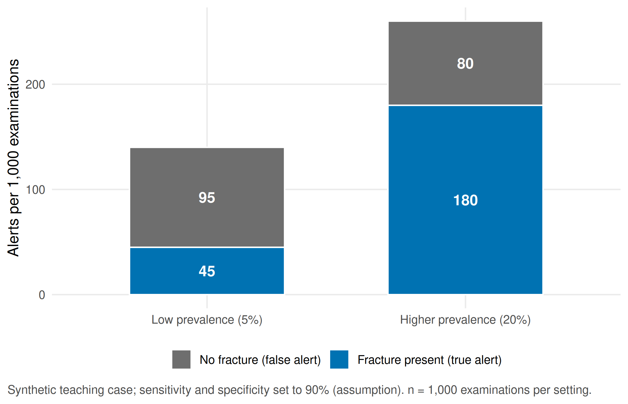
Report. In the low-prevalence setting, 45 of 140 alerts concern a fracture (PPV 32.1%); in the higher-prevalence setting it is 180 of 260 (69.2%). A defensible handover sentence for the first setting reads: “In our teaching scenario about one in three alerts was a fracture; the image is re-read in its clinical context.” The lower PPV alone is no reason to reject a tool. Whether the second look improves treatment is a different question that needs a comparison group and patient-relevant outcomes.
TipCounter-check: predict first
Specificity improves from 90% to 95% in the low-prevalence setting, sensitivity stays at 90%. Will the PPV rise to about 40%, 50% or 60%? Write down your guess, then run the chunk.
# Counter-check: predict first, then compute. Specificity rises from 90% to 95% at 5% prevalence.
fp_new  <- (1 - 0.95) * 950
ppv_new <- 45 / (45 + fp_new)
cat("False alerts:", fp_new, " PPV:", cdsr_percent(ppv_new), "\n")
#> False alerts: 47.5 PPV: 48.6%stopifnot(isTRUE(all.equal(fp_new, 47.5)), identical(cdsr_percent(ppv_new), "48.6%"))Part B · A baseline and an alternative on the same test patients (unit 10)
Decision. The team wants to know whether a more complex model ranks patients better than a simple logistic regression with four predictors chosen in advance. Both are judged on the same, fixed test patients.
Look at the data. The synthetic cohort has 2,000 admissions with suspected wrist fracture. The reference standard (fracture yes or no) is known for everyone. 600 admissions are drawn once as the test set; their identifiers are stored with the data, so another group can reproduce exactly the same split.
# Part B (unit 10): synthetic emergency department admissions with suspected wrist fracture
set.seed(20260309)
n <- 2000
cohort <- data.frame(id = sprintf("ED%04d", seq_len(n)))
cohort$age <- round(runif(n, 18, 95))                                  # years
cohort$age_group <- factor(ifelse(cohort$age >= 75, "75 and older", "18 to 74"),
                           levels = c("18 to 74", "75 and older"))
cohort$fall_outstretched <- rbinom(n, 1, 0.55)                         # fall on outstretched hand (0/1)
# Reference standard (fracture yes/no) depends on age and mechanism
lp <- -2.6 + 0.02 * (cohort$age - 50) + 1.0 * cohort$fall_outstretched
cohort$fracture <- rbinom(n, 1, plogis(lp))
# Clinical signs: in older patients both signs are weaker indicators (synthetic assumption)
older <- cohort$age_group == "75 and older"
cohort$snuffbox_tender <- rbinom(n, 1, ifelse(cohort$fracture == 1, ifelse(older, 0.55, 0.80), 0.25))
cohort$swelling        <- rbinom(n, 1, ifelse(cohort$fracture == 1, ifelse(older, 0.45, 0.80), 0.20))
cohort$grip_kg <- round(rnorm(n, 32 - 0.15 * (cohort$age - 50) - 5 * cohort$fracture, 6), 1)
cohort$grip_kg[sample(n, 100)] <- NA                                   # 5% not measured
cohort$noise <- round(rnorm(n), 2)                                     # unrelated variable

# Fixed test set: 600 admissions drawn once and stored with the data
test_ids <- sort(sample(cohort$id, 600))
cohort$split <- ifelse(cohort$id %in% test_ids, "test", "train")
train <- cohort[cohort$split == "train", ]
test  <- cohort[cohort$split == "test", ]
stopifnot(nrow(train) == 1400, nrow(test) == 600,
          length(intersect(train$id, test$id)) == 0)
table(split = cohort$split, fracture = cohort$fracture)
#> fracture
#> split 0 1
#> test 516 84
#> train 1180 220Assumption. Grip strength is missing for 5% of admissions. Any pre-processing step, here the median used to fill in missing grip strength, is learnt from the training data only and then applied unchanged to the test set. Using the median of all 2,000 admissions would leak information from the test set into the model.
# Pre-processing uses training data only: the training median replaces missing grip strength
grip_median_train <- median(train$grip_kg, na.rm = TRUE)
impute_grip <- function(d) {
  d$grip_missing <- as.integer(is.na(d$grip_kg))
  d$grip_kg[is.na(d$grip_kg)] <- grip_median_train
  d
}
train <- impute_grip(train)
test  <- impute_grip(test)
grip_median_train
#> [1] 30.3The alternative model is an elastic net with all variables and all pairwise interactions. Its penalty is tuned by five-fold cross-validation inside the training data; the test set is touched once, at the end.
# Null model: everyone receives the training prevalence
p_null <- mean(train$fracture)
# Baseline: logistic regression with four pre-specified predictors
baseline <- glm(fracture ~ age + fall_outstretched + snuffbox_tender + swelling,
                family = binomial, data = train)
# Alternative: elastic net with all variables and their pairwise interactions;
# the penalty is tuned by 5-fold cross-validation inside the training data only
f_alt <- ~ (age + fall_outstretched + snuffbox_tender + swelling + grip_kg + grip_missing + noise)^2
x_train <- model.matrix(f_alt, train)[, -1]
x_test  <- model.matrix(f_alt, test)[, -1]
fold_id <- rep_len(1:5, nrow(train))[order(train$id)]      # fixed, reproducible folds
alt_fit <- cv.glmnet(x_train, train$fracture, family = "binomial", alpha = 0.5, foldid = fold_id)

test$p_null     <- p_null
test$p_baseline <- predict(baseline, newdata = test, type = "response")
test$p_alt      <- as.numeric(predict(alt_fit, newx = x_test, s = "lambda.1se", type = "response"))

# Performance on the fixed test set
brier <- function(p, y) mean((p - y)^2)
calib <- function(p, y) {                       # calibration intercept and slope
  lp <- qlogis(pmin(pmax(p, 1e-6), 1 - 1e-6))
  c(intercept = unname(coef(glm(y ~ offset(lp), family = binomial))[1]),
    slope = unname(coef(glm(y ~ lp, family = binomial))[2]))
}
results <- data.frame(
  model = c("Null model (training prevalence)", "Baseline: logistic regression, 4 predictors",
            "Alternative: elastic net with interactions"),
  n_test = nrow(test), fractures_test = sum(test$fracture),
  auc   = c(0.5, auc_rank(test$p_baseline, test$fracture), auc_rank(test$p_alt, test$fracture)),
  brier = c(brier(test$p_null, test$fracture), brier(test$p_baseline, test$fracture),
            brier(test$p_alt, test$fracture)),
  calib_slope = c(NA, calib(test$p_baseline, test$fracture)["slope"],
                  calib(test$p_alt, test$fracture)["slope"])
)
print(results, digits = 3)
#> model n_test fractures_test auc
#> 1 Null model (training prevalence) 600 84 0.500
#> 2 Baseline: logistic regression, 4 predictors 600 84 0.858
#> 3 Alternative: elastic net with interactions 600 84 0.883
#> brier calib_slope
#> 1 0.1207 NA
#> 2 0.0907 0.86
#> 3 0.0803 1.18stopifnot(
results$n_test[1] == 600,
all(results$auc[2:3] > 0.65 & results$auc[2:3] < 0.95),
all(results$brier[2:3] < results$brier[1]), # both models beat the null model
abs(results$auc[3] - results$auc[2]) < 0.05 # small gain in ranking for considerably more effort
)knitr::kable(results[, c("model", "n_test", "fractures_test", "auc", "brier", "calib_slope")],
digits = 3, col.names = c("Model", "Test admissions", "Fractures", "AUC", "Brier score",
"Calibration slope"))| Model | Test admissions | Fractures | AUC | Brier score | Calibration slope |
|---|---|---|---|---|---|
| Null model (training prevalence) | 600 | 84 | 0.500 | 0.121 | NA |
| Baseline: logistic regression, 4 predictors | 600 | 84 | 0.858 | 0.091 | 0.860 |
| Alternative: elastic net with interactions | 600 | 84 | 0.883 | 0.080 | 1.182 |
Report. On the same 600 test admissions, the baseline reaches an AUC of 0.858 and the elastic net 0.883. The difference in ranking is small compared with the additional effort for tuning, documentation and maintenance; whether it matters depends on the decision the score is meant to support, which Part C makes concrete.
Part C · Calibration, threshold and who carries the errors (unit 11)
Decision. At which predicted risk should the tool raise an alert, and which group pays for that choice in missed fractures or unnecessary extra imaging?
# Part C (unit 11): calibration by fifths of predicted risk in the test set
calib_bins <- function(p, y, model) {
  bin <- cut(p, quantile(p, probs = seq(0, 1, 0.2)), include.lowest = TRUE, labels = FALSE)
  do.call(rbind, lapply(split(data.frame(p, y), bin), function(d) {
    ci <- prop_ci(sum(d$y), nrow(d))
    data.frame(model = model, predicted = mean(d$p), observed = ci[["estimate"]],
               lower = ci[["lower"]], upper = ci[["upper"]], n = nrow(d))
  }))
}
calib_df <- rbind(calib_bins(test$p_baseline, test$fracture, "Baseline"),
                  calib_bins(test$p_alt, test$fracture, "Elastic net"))
p_calib <- ggplot(calib_df, aes(predicted, observed, colour = model, shape = model)) +
  geom_abline(slope = 1, intercept = 0, linetype = "22", colour = "grey50") +
  geom_pointrange(aes(ymin = lower, ymax = upper)) +
  geom_line(aes(linetype = model)) +
  scale_colour_manual(values = unname(cdsr_colours[c("blue", "orange")])) +
  scale_shape_manual(values = cdsr_shapes[1:2]) +
  scale_linetype_manual(values = cdsr_linetypes[1:2]) +
  scale_x_continuous(labels = scales::percent, limits = c(0, NA)) +
  scale_y_continuous(labels = scales::percent, limits = c(0, NA)) +
  labs(x = "Mean predicted risk in the group", y = "Observed share with fracture (95% CI)",
       colour = NULL, shape = NULL, linetype = NULL,
       caption = "Synthetic test set, n = 600 admissions in five groups of 120 per model; dashed line = perfect calibration.") +
  theme_cdsr()
show_figure(p_calib, "w3-calibration.png")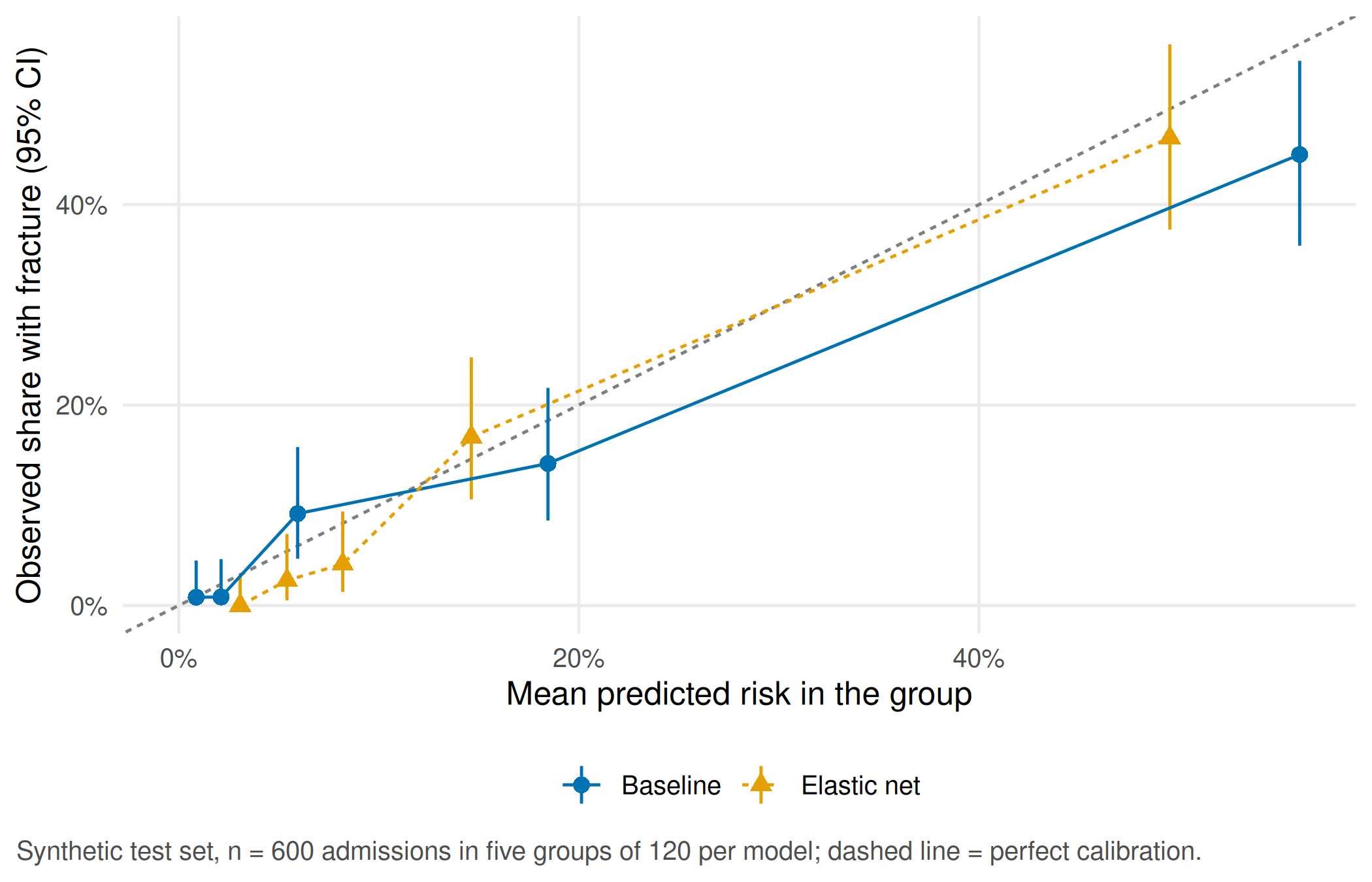
A good AUC says that patients with fractures tend to receive higher scores. It does not say that a predicted risk of 50% means that half of these patients have a fracture. The calibration plot answers that second question.
Now move the threshold. The shift size of 30 wrist examinations is an assumption used to translate rates into a workload that clinicians recognise.
# Moving the threshold for the baseline model; 30 wrist examinations per shift (assumption)
per_shift <- 30
threshold_table <- do.call(rbind, lapply(c(0.10, 0.20, 0.30, 0.40), function(t) {
  alert <- test$p_baseline >= t
  y <- test$fracture == 1
  data.frame(threshold = t, alerts = sum(alert), tp = sum(alert & y), fp = sum(alert & !y),
             fn = sum(!alert & y), sensitivity = mean(alert[y]), specificity = mean(!alert[!y]),
             ppv = sum(alert & y) / sum(alert),
             false_alerts_per_shift = per_shift * sum(alert & !y) / nrow(test))
}))
print(threshold_table, digits = 3)
#> threshold alerts tp fp fn sensitivity specificity ppv
#> 1 0.1 240 71 169 13 0.845 0.672 0.296
#> 2 0.2 163 60 103 24 0.714 0.800 0.368
#> 3 0.3 124 54 70 30 0.643 0.864 0.435
#> 4 0.4 92 47 45 37 0.560 0.913 0.511
#> false_alerts_per_shift
#> 1 8.45
#> 2 5.15
#> 3 3.50
#> 4 2.25stopifnot(all(diff(threshold_table$alerts) <= 0), # higher threshold, fewer alerts
all(diff(threshold_table$sensitivity) <= 0)) # ... and fewer fractures detectedFinally, look at errors by age group at an example threshold of 20%. Every rate is given with its denominator and an exact 95% confidence interval.
# Errors by age group at the example threshold of 20%, with denominators and exact 95% intervals
threshold <- 0.20
test$alert <- test$p_baseline >= threshold
subgroup_table <- do.call(rbind, lapply(split(test, test$age_group), function(d) {
  y <- d$fracture == 1
  data.frame(age_group = d$age_group[1], admissions = nrow(d), fractures = sum(y),
             detected = format_prop(sum(d$alert & y), sum(y)),
             missed = sum(!d$alert & y),
             false_alerts = format_prop(sum(d$alert & !y), sum(!y)))
}))
print(subgroup_table, row.names = FALSE)
#> age_group admissions fractures detected missed
#> 18 to 74 431 46 35/46 = 76.1% (61.2% to 87.4%) 11
#> 75 and older 169 38 25/38 = 65.8% (48.6% to 80.4%) 13
#> false_alerts
#> 60/385 = 15.6% (12.1% to 19.6%)
#> 43/131 = 32.8% (24.9% to 41.6%)sens_by_group <- tapply(test$alert[test$fracture == 1], test$age_group[test$fracture == 1], mean)
stopifnot(sens_by_group[["75 and older"]] < sens_by_group[["18 to 74"]])Report. At a threshold of 20%, the tool detects 35/46 = 76.1% (61.2% to 87.4%) of fractures in people aged 18 to 74 but only 25/38 = 65.8% (48.6% to 80.4%) in people aged 75 and older, and it raises false alerts for 43/131 = 32.8% (24.9% to 41.6%) of older people without a fracture. In this synthetic cohort, older patients carry both more missed fractures and more unnecessary follow-up. The intervals overlap for sensitivity, so the difference needs confirmation; the information missing to decide is the size and direction of this gap in real local data.
WarningCommon mistake
Reporting “sensitivity 71%” without the number of fractures behind it. With 38 fractures in a subgroup the 95% interval spans more than 30 percentage points. Always give x/n.
Your record for the workshop
- Two two-by-two tables (Part A) with all eight cells and both PPVs.
- The results table (Part B) with the test denominator and a sentence on whether the extra effort is justified.
- A threshold you would propose for the pilot, the group that is disadvantaged by it, and the one piece of information you would need before deciding (Part C).
Download the tables linked at the top if you want to continue in a spreadsheet. The script writes the same files to output/ when you run it on your own.
Further reading
- Companion book: B06 · Accuracy, calibration and clinical utility and B09 · A fracture alert in the emergency department – the case behind Part A.
- Methods in R: Predictive Values and Prevalence – the general formulae and their pitfalls.
- Methods in R: Calibration Plots – more ways to draw and test calibration.
- CTTIR Courses: Logistic regression (binomial GLM) – the baseline model step by step.
- CTTIR Tutorials: Cutpoint Selection – why a threshold is a decision, not a property of the model.