library(ggplot2)
library(deSolve)
library(simmer)Lab W6 · Forecast, PK, queue and priors
Teaching units 21–23: a forecast of emergency department arrivals tested on later weeks, two elective simulation stations (pharmacokinetics or operating capacity in a mass casualty incident) and a small binomial result under two priors.
Every part of this lab follows the same five steps: state the decision, look at the data, name the assumption, compute in R and write one sentence for the person who has to act. All numbers are synthetic or teaching assumptions. The pharmacokinetic example uses virtual parameters for one virtual individual; it names no drug and contains no dosing recommendation.
Part A is for everyone. In Part B each group works through one station (pharmacokinetics or operating capacity) completely and reviews the other station from its printed curves and tables. Part C is again for everyone. If R is new to you, read the code and the printed output first; the results on this page are complete. If you are fluent in R, run the counter-checks before reading their output.
Part A · Is next week’s forecast usable for staffing? (unit 21)
Decision. A fictitious emergency department plans nursing staff per shift one week ahead. The team asks whether a simple forecast of hourly arrivals, with an interval, is good enough to plan the next week, and in which shift a wrong forecast would hurt patients most.
Look at the data. The synthetic department records arrivals per hour for 16 weeks. There is a daily rhythm (quiet at night, busy in the early afternoon), a weekly rhythm (busier on Mondays, quieter at weekends) and, from week 13, a winter wave with 25% more arrivals (assumption). The forecasting rules below do not know about the wave.
# Part A (unit 21): synthetic hourly arrivals at an emergency department over 16 weeks
set.seed(20260321)
n_weeks <- 16
hour_index <- 0:(n_weeks * 168 - 1)                       # 168 hours per week
ed <- data.frame(
  index        = hour_index + 1,
  week         = hour_index %/% 168 + 1,
  hour_of_week = hour_index %% 168 + 1,
  day          = hour_index %/% 24 + 1,
  hour         = hour_index %% 24                         # 0 = midnight to 1 a.m.
)
weekday_names <- c("Mon", "Tue", "Wed", "Thu", "Fri", "Sat", "Sun")
ed$weekday <- factor(weekday_names[(ed$day - 1) %% 7 + 1], levels = weekday_names)
# Expected arrivals per hour: daily profile x weekday factor x winter wave (all assumptions)
daily_profile  <- 2 + 7 * exp(-(ed$hour - 13)^2 / (2 * 4^2))          # low at night, peak early afternoon
weekday_factor <- c(1.15, 1.05, 1.00, 1.00, 1.05, 0.90, 0.85)[as.integer(ed$weekday)]
wave_factor    <- ifelse(ed$week >= 13, 1.25, 1)                       # +25% from week 13
ed$expected <- daily_profile * weekday_factor * wave_factor
ed$arrivals <- rpois(nrow(ed), ed$expected)
ed$shift <- factor(ifelse(ed$hour >= 22 | ed$hour < 6, "Night (22-06)",
                          ifelse(ed$hour < 14, "Early (06-14)", "Late (14-22)")),
                   levels = c("Night (22-06)", "Early (06-14)", "Late (14-22)"))
stopifnot(nrow(ed) == 2688, sum(ed$arrivals) > 0)
daily_totals <- aggregate(arrivals ~ day + week, data = ed, FUN = sum)
summary(daily_totals$arrivals)
#> Min. 1st Qu. Median Mean 3rd Qu. Max.
#> 80.0 112.0 123.0 126.1 135.2 190.0p_arrivals <- ggplot(daily_totals, aes(day, arrivals)) +
geom_vline(xintercept = 12 * 7 + 0.5, linetype = "22", colour = cdsr_colours[["grey"]]) +
annotate("text", x = 12 * 7 - 0.5, y = max(daily_totals$arrivals), hjust = 1, size = 3.5,
label = "Winter wave from week 13 (assumption) →") +
geom_line(colour = cdsr_colours[["blue"]]) +
geom_point(colour = cdsr_colours[["blue"]], size = 1) +
scale_x_continuous(breaks = seq(1, 113, by = 14), name = "Day of the observation period") +
labs(y = "Arrivals per day",
caption = "Synthetic emergency department; n = 112 days (2,688 hours) from one fictitious department.") +
theme_cdsr()
show_figure(p_arrivals, "w6-arrivals.png")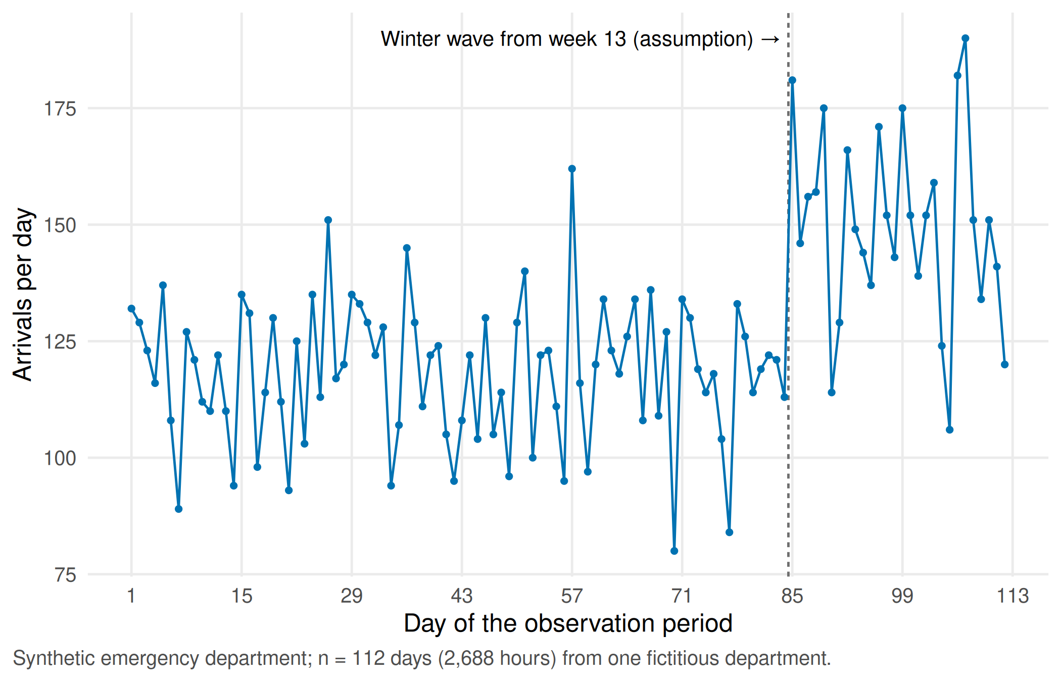
Assumption. Both rules assume that the coming week resembles the recent past. The baseline repeats the same hour of the previous week (“seasonal naive”); the alternative averages the same hour over the last four weeks. Each 80% interval is learnt from the rule’s own errors in the four weeks before the forecast origin, so it assumes that future errors look like past errors.
Compute. The forecasts are evaluated only on weeks that lie after the forecast origin (rolling origin): for week 9 the rules see weeks 1–8, for week 10 weeks 1–9, and so on up to week 16. The stopifnot() line checks that no forecast uses an hour at or after its own origin.
# Two forecasting rules for the next 168 hours; both see only the history before the origin
forecast_week <- function(history, method) {
  n <- length(history)
  if (method == "Same hour last week") {
    history[(n - 167):n]                                          # seasonal naive baseline
  } else {
    rowMeans(matrix(history[(n - 4 * 168 + 1):n], nrow = 168))    # mean of the same hour, last 4 weeks
  }
}
# Errors of the same rule in the four weeks before the origin give an empirical 80% interval
past_errors <- function(history, method) {
  n <- length(history)
  unlist(lapply(1:4, function(k) {
    cut <- n - k * 168
    history[(cut + 1):(cut + 168)] - forecast_week(history[seq_len(cut)], method)
  }))
}
methods <- c("Same hour last week", "Mean of last 4 weeks")
origins <- 9:16                                                    # forecast origin = Monday 00:00 of week 9 ... 16
forecasts <- do.call(rbind, lapply(origins, function(w) {
  origin <- (w - 1) * 168 + 1                                      # index of the first forecast hour
  history <- ed$arrivals[seq_len(origin - 1)]                      # nothing at or after the origin
  do.call(rbind, lapply(methods, function(m) {
    point <- forecast_week(history, m)
    q <- quantile(past_errors(history, m), c(0.10, 0.90), names = FALSE)
    data.frame(method = m, origin_week = w, horizon = 1:168,
               target_index = origin:(origin + 167), history_end = length(history),
               forecast = point, lower = pmax(point + q[1], 0), upper = point + q[2])
  }))
}))
forecasts$observed <- ed$arrivals[forecasts$target_index]
forecasts$shift    <- ed$shift[forecasts$target_index]
forecasts$period   <- ifelse(forecasts$origin_week >= 13, "Weeks 13-16 (wave)", "Weeks 9-12 (before wave)")
forecasts$error    <- forecasts$observed - forecasts$forecast      # positive = under-forecast
forecasts$covered  <- forecasts$observed >= forecasts$lower & forecasts$observed <= forecasts$upper
forecasts$horizon_band <- cut(forecasts$horizon, c(0, 24, 72, 168),
                              labels = c("1-24 h", "25-72 h", "73-168 h"))
# The forecast never uses data from the forecast window or later
stopifnot(all(forecasts$history_end < forecasts$target_index),
          nrow(forecasts) == length(origins) * length(methods) * 168)
evaluate <- function(d) data.frame(hours = nrow(d), mae = mean(abs(d$error)),
mean_error = mean(d$error), coverage_80 = mean(d$covered))
eval_period <- do.call(rbind, lapply(split(forecasts, list(forecasts$method, forecasts$period)), function(d)
cbind(method = d$method[1], period = d$period[1], evaluate(d))))
eval_horizon <- do.call(rbind, lapply(split(forecasts, list(forecasts$method, forecasts$horizon_band)), function(d)
cbind(method = d$method[1], horizon = as.character(d$horizon_band[1]), evaluate(d))))
eval_period <- eval_period[order(eval_period$method, eval_period$period), ]
eval_horizon <- eval_horizon[order(eval_horizon$method, eval_horizon$horizon), ]
rownames(eval_period) <- rownames(eval_horizon) <- NULL
print(eval_period, digits = 3)#> method period hours mae mean_error
#> 1 Mean of last 4 weeks Weeks 13-16 (wave) 672 2.18 0.8065
#> 2 Mean of last 4 weeks Weeks 9-12 (before wave) 672 1.83 0.0685
#> 3 Same hour last week Weeks 13-16 (wave) 672 2.63 0.3289
#> 4 Same hour last week Weeks 9-12 (before wave) 672 2.26 0.0417
#> coverage_80
#> 1 0.783
#> 2 0.810
#> 3 0.824
#> 4 0.878print(eval_horizon, digits = 3)#> method horizon hours mae mean_error coverage_80
#> 1 Mean of last 4 weeks 1-24 h 192 2.10 0.652 0.771
#> 2 Mean of last 4 weeks 25-72 h 384 2.05 0.485 0.805
#> 3 Mean of last 4 weeks 73-168 h 768 1.96 0.360 0.798
#> 4 Same hour last week 1-24 h 192 2.55 0.276 0.828
#> 5 Same hour last week 25-72 h 384 2.49 0.263 0.854
#> 6 Same hour last week 73-168 h 768 2.40 0.124 0.855# Under-forecast per 8-hour shift during the wave: missing arrivals per shift, averaged over shifts
wave <- forecasts[forecasts$period == "Weeks 13-16 (wave)", ]
shift_gap <- aggregate(error ~ method + shift, data = wave, FUN = function(e) sum(e) / (length(e) / 8))
names(shift_gap)[3] <- "under_forecast_per_shift"
print(shift_gap, digits = 3)#> method shift under_forecast_per_shift
#> 1 Mean of last 4 weeks Night (22-06) 4.76
#> 2 Same hour last week Night (22-06) 2.71
#> 3 Mean of last 4 weeks Early (06-14) 6.45
#> 4 Same hour last week Early (06-14) 1.61
#> 5 Mean of last 4 weeks Late (14-22) 8.15
#> 6 Same hour last week Late (14-22) 3.57stopifnot(
all(eval_period$hours == 4 * 168), # each cell: 672 forecast hours
sum(eval_horizon$hours) == 2 * 8 * 168, # 2 methods x 8 weeks x 168 hours
# before the wave, averaging four weeks beats last week's value
eval_period$mae[eval_period$method == "Mean of last 4 weeks" & eval_period$period == "Weeks 9-12 (before wave)"] <
eval_period$mae[eval_period$method == "Same hour last week" & eval_period$period == "Weeks 9-12 (before wave)"],
# during the wave, both rules under-forecast on average
all(eval_period$mean_error[eval_period$period == "Weeks 13-16 (wave)"] > 0)
)
# The largest gap per shift: the late shift with the 4-week mean
gap_mean4 <- shift_gap[shift_gap$method == "Mean of last 4 weeks", ]
stopifnot(as.character(gap_mean4$shift[which.max(gap_mean4$under_forecast_per_shift)]) == "Late (14-22)")knitr::kable(eval_period, digits = 2,
col.names = c("Rule", "Period", "Hours", "MAE (arrivals/h)", "Mean error (arrivals/h)",
"80% interval coverage"))| Rule | Period | Hours | MAE (arrivals/h) | Mean error (arrivals/h) | 80% interval coverage |
|---|---|---|---|---|---|
| Mean of last 4 weeks | Weeks 13-16 (wave) | 672 | 2.18 | 0.81 | 0.78 |
| Mean of last 4 weeks | Weeks 9-12 (before wave) | 672 | 1.83 | 0.07 | 0.81 |
| Same hour last week | Weeks 13-16 (wave) | 672 | 2.63 | 0.33 | 0.82 |
| Same hour last week | Weeks 9-12 (before wave) | 672 | 2.26 | 0.04 | 0.88 |
week13 <- forecasts[forecasts$origin_week == 13, ]
week13$hour_label <- week13$horizon
p_forecast <- ggplot(week13, aes(horizon)) +
  geom_ribbon(data = week13[week13$method == "Mean of last 4 weeks", ],
              aes(ymin = lower, ymax = upper), fill = cdsr_colours[["orange"]], alpha = 0.2) +
  geom_point(data = week13[week13$method == "Mean of last 4 weeks", ], aes(y = observed),
             colour = "grey30", size = 0.8) +
  geom_line(aes(y = forecast, colour = method, linetype = method)) +
  scale_colour_manual(values = unname(cdsr_colours[c("orange", "blue")])) +
  scale_linetype_manual(values = cdsr_linetypes[1:2]) +
  scale_x_continuous(breaks = seq(1, 169, by = 24), labels = weekday_names[c(1:7, 1)][1:8],
                     name = "Hour of the forecast week (week 13, first week of the wave)") +
  labs(y = "Arrivals per hour", colour = NULL, linetype = NULL,
       caption = "Points: observed arrivals; band: 80% interval of the 4-week mean. Synthetic data; n = 168 hours.") +
  theme_cdsr()
show_figure(p_forecast, "w6-forecast-week.png")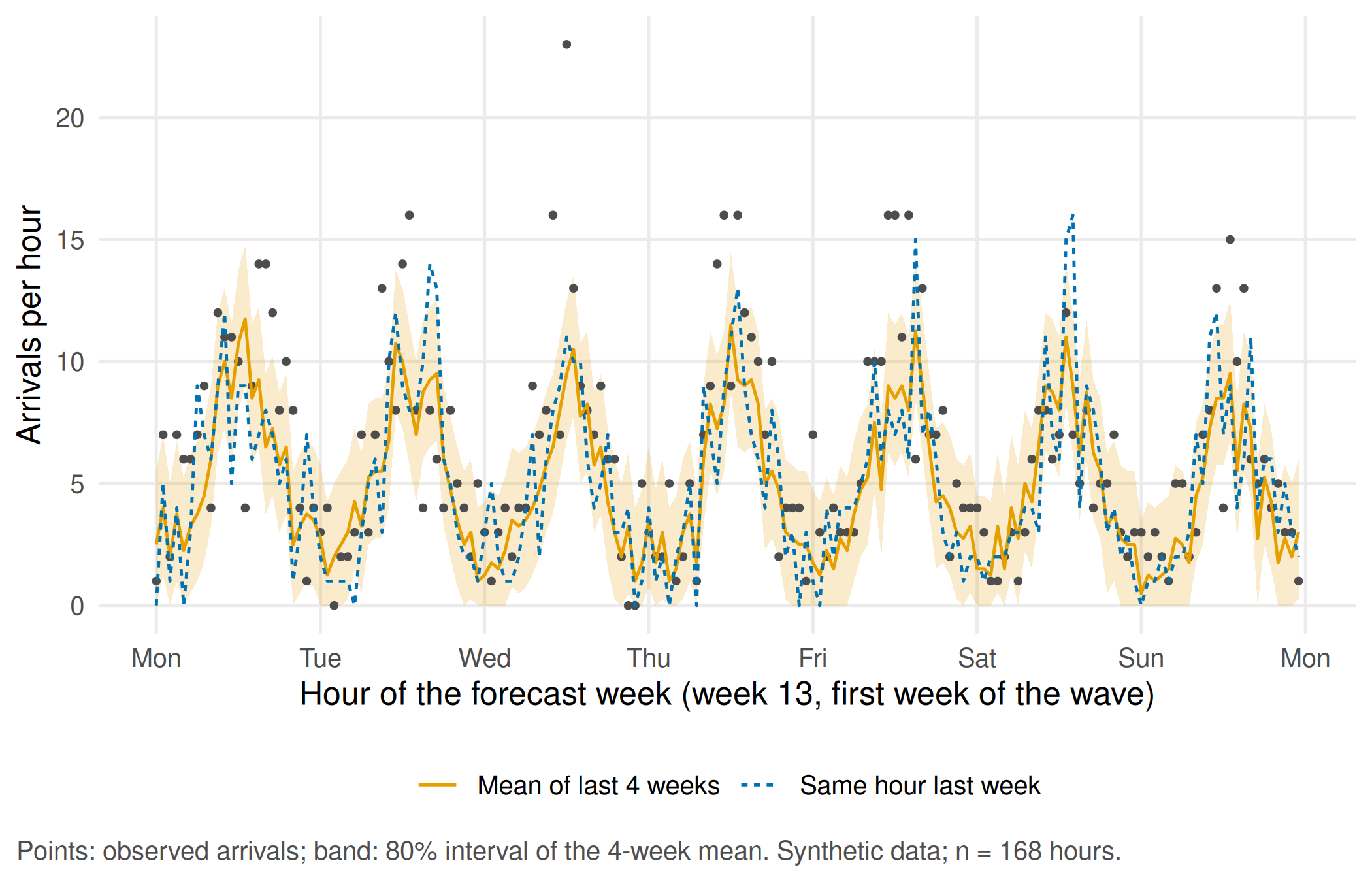
Report. Before the wave, the 4-week mean is the more precise rule (MAE 1.83 against 2.26 arrivals per hour) and its 80% interval covers 81.0% of hours. During the wave it under-forecasts by 0.81 arrivals per hour on average (the baseline by 0.33), coverage falls to 78.3%, and the gap concentrates in the late shift: about 8.2 arrivals per late shift were not forecast, against 4.8 per night shift. A sentence for the nurse manager: “The forecast is usable for normal weeks; after a sudden rise it lags for several weeks, so a rise of this size should trigger a manual review of the late shift rather than rely on the interval.” The interval describes uncertainty only under the assumption that the process has not changed.
The table by horizon shows a second point: for these weekly rules, the error barely grows from the first day to the seventh. What matters more is how long ago the level last changed.
knitr::kable(eval_horizon, digits = 2,
             col.names = c("Rule", "Horizon", "Hours", "MAE (arrivals/h)", "Mean error (arrivals/h)",
"80% interval coverage"))| Rule | Horizon | Hours | MAE (arrivals/h) | Mean error (arrivals/h) | 80% interval coverage |
|---|---|---|---|---|---|
| Mean of last 4 weeks | 1-24 h | 192 | 2.10 | 0.65 | 0.77 |
| Mean of last 4 weeks | 25-72 h | 384 | 2.05 | 0.49 | 0.80 |
| Mean of last 4 weeks | 73-168 h | 768 | 1.96 | 0.36 | 0.80 |
| Same hour last week | 1-24 h | 192 | 2.55 | 0.28 | 0.83 |
| Same hour last week | 25-72 h | 384 | 2.49 | 0.26 | 0.85 |
| Same hour last week | 73-168 h | 768 | 2.40 | 0.12 | 0.86 |
TipCounter-check: predict first
In week 14 the wave has been running for one week. Which rule will now have the smaller average under-forecast, and why? Write down your answer, then run the chunk.
# Counter-check: mean error (observed - forecast) per forecast week. Which rule recovers after the jump?
by_week <- aggregate(error ~ origin_week + method, data = forecasts, FUN = mean)
by_week <- reshape(by_week, idvar = "origin_week", timevar = "method", direction = "wide")
names(by_week) <- c("forecast_week", "mean_error_4_week_mean", "mean_error_last_week")
print(by_week[by_week$forecast_week >= 12, ], digits = 2, row.names = FALSE)
#> forecast_week mean_error_4_week_mean mean_error_last_week
#> 12 0.12 0.268
#> 13 1.33 1.250
#> 14 1.07 0.024
#> 15 0.38 -0.327
#> 16 0.45 0.369# From week 14 on, last week's value already contains the wave; the 4-week mean still lags
stopifnot(all(by_week$mean_error_last_week[by_week$forecast_week >= 14] <
by_week$mean_error_4_week_mean[by_week$forecast_week >= 14]))
WarningCommon mistake
Evaluating a forecast on randomly chosen hours, or computing the “mean of the last four weeks” with weeks that lie after the hour to be forecast. Both let the future leak into the forecast and make it look better than it can be in practice. Time series are tested only on periods that come later than everything the rule has seen.
Part B · Two elective simulation stations (unit 22)
Station PK · Does the solver reproduce the known answer?
Decision. A research group plans a pharmacokinetic sampling scheme and wants to use a numerical solver for more complex models later. Before trusting the solver, it must reproduce a case whose answer is known exactly.
Assumption. One compartment, first-order elimination after an intravenous bolus, virtual parameters: clearance CL = 5 L/h, volume of distribution V = 50 L, virtual amount 100 mg (assumption; no drug, no dosing recommendation). The analytic solution is \(C(t) = \frac{\text{Dose}}{V}\, e^{-\frac{CL}{V} t}\) in mg/L. Units and tolerance are fixed before computing: time in hours, concentration in mg/L, and the numerical and analytic concentrations at the same 49 time points (0 to 24 h every 30 minutes) may differ by at most a relative \(10^{-6}\) (the value of tolerance in the code).
# Part B, station PK (unit 22): one-compartment model after an intravenous bolus.
# Virtual parameters for a teaching exercise only (no drug, no dosing recommendation).
dose  <- 100                          # mg, virtual amount
base  <- c(CL = 5, V = 50)            # clearance in L/h, volume of distribution in L
times <- seq(0, 24, by = 0.5)         # h, identical time points for both methods
tolerance <- 1e-6                     # maximal relative difference, fixed before computing

analytic_conc <- function(p) dose / p[["V"]] * exp(-p[["CL"]] / p[["V"]] * times)   # mg/L
one_compartment <- function(t, state, p) list(-p[["CL"]] / p[["V"]] * state[["A"]])  # dA/dt in mg/h
ode_conc <- function(p) {
  out <- ode(y = c(A = dose), times = times, func = one_compartment, parms = p,
             method = "lsoda", rtol = 1e-10, atol = 1e-12)
  out[, "A"] / p[["V"]]                                                              # amount / volume
}
c_ode <- ode_conc(base)
c_ana <- analytic_conc(base)
max_rel_diff <- max(abs(c_ode - c_ana) / c_ana)
half_life <- log(2) * base[["V"]] / base[["CL"]]                                     # h
auc_inf   <- dose / base[["CL"]]                                                     # mg*h/L
cat("Max. relative difference ODE vs analytic:", signif(max_rel_diff, 2),
    "\nHalf-life:", round(half_life, 2), "h   C(0):", dose / base[["V"]], "mg/L   AUC(0-inf):", auc_inf, "mg*h/L\n")
#> Max. relative difference ODE vs analytic: 1.5e-10
#> Half-life: 6.93 h C(0): 2 mg/L AUC(0-inf): 20 mg*h/Lstopifnot(max_rel_diff < tolerance, round(half_life, 2) == 6.93,
isTRUE(all.equal(c_ana[1], 2)), isTRUE(all.equal(auc_inf, 20)))
# Vary one parameter at a time
pk_scenarios <- data.frame(
varied = c("Reference", "Clearance", "Clearance", "Volume", "Volume"),
CL = c(5, 2.5, 10, 5, 5),
V = c(50, 50, 50, 25, 100)
)
pk_scenarios$c0_mg_per_l <- dose / pk_scenarios$V
pk_scenarios$half_life_h <- log(2) * pk_scenarios$V / pk_scenarios$CL
pk_scenarios$c12_mg_per_l <- dose / pk_scenarios$V * exp(-pk_scenarios$CL / pk_scenarios$V * 12)
pk_scenarios$auc_mg_h_per_l <- dose / pk_scenarios$CL
print(pk_scenarios, digits = 3)#> varied CL V c0_mg_per_l half_life_h c12_mg_per_l auc_mg_h_per_l
#> 1 Reference 5.0 50 2 6.93 0.602 20
#> 2 Clearance 2.5 50 2 13.86 1.098 40
#> 3 Clearance 10.0 50 2 3.47 0.181 10
#> 4 Volume 5.0 25 4 3.47 0.363 20
#> 5 Volume 5.0 100 1 13.86 0.549 20pk_curves <- do.call(rbind, lapply(seq_len(nrow(pk_scenarios)), function(i) {
p <- c(CL = pk_scenarios$CL[i], V = pk_scenarios$V[i])
data.frame(scenario = sprintf("CL %s L/h, V %s L", p[["CL"]], p[["V"]]), time_h = times,
conc_ode = ode_conc(p), conc_analytic = analytic_conc(p))
}))
stopifnot(max(abs(pk_curves$conc_ode - pk_curves$conc_analytic) / pk_curves$conc_analytic) < tolerance)curve_panels <- rbind(
cbind(pk_curves[pk_curves$scenario %in% c("CL 2.5 L/h, V 50 L", "CL 5 L/h, V 50 L", "CL 10 L/h, V 50 L"), ],
panel = "Clearance varied (V = 50 L)"),
cbind(pk_curves[pk_curves$scenario %in% c("CL 5 L/h, V 25 L", "CL 5 L/h, V 50 L", "CL 5 L/h, V 100 L"), ],
panel = "Volume varied (CL = 5 L/h)")
)
curve_panels$role <- ifelse(curve_panels$scenario == "CL 5 L/h, V 50 L", "Reference",
ifelse(grepl("CL 2.5|V 25 L", curve_panels$scenario), "Halved", "Doubled"))
curve_panels$role <- factor(curve_panels$role, levels = c("Halved", "Reference", "Doubled"))
p_pk <- ggplot(curve_panels, aes(time_h, conc_ode, colour = role, linetype = role)) +
geom_line(linewidth = 0.8) +
geom_point(data = curve_panels[curve_panels$time_h %% 4 == 0, ], aes(y = conc_analytic, shape = role),
size = 1.8) +
facet_wrap(~ panel) +
scale_y_log10() +
scale_colour_manual(values = unname(cdsr_colours[c("orange", "blue", "green")])) +
scale_linetype_manual(values = cdsr_linetypes[c(2, 1, 3)]) +
scale_shape_manual(values = cdsr_shapes[c(2, 1, 3)]) +
labs(x = "Time after the virtual bolus (h)", y = "Concentration (mg/L, log scale)",
colour = "Parameter", linetype = "Parameter", shape = "Parameter",
caption = paste("Lines: numerical solution (deSolve); points: analytic solution every 4 h.",
"Virtual parameters, one virtual individual; no dosing recommendation.", sep = "\n")) +
theme_cdsr()
show_figure(p_pk, "w6-pk.png", width = 7.5)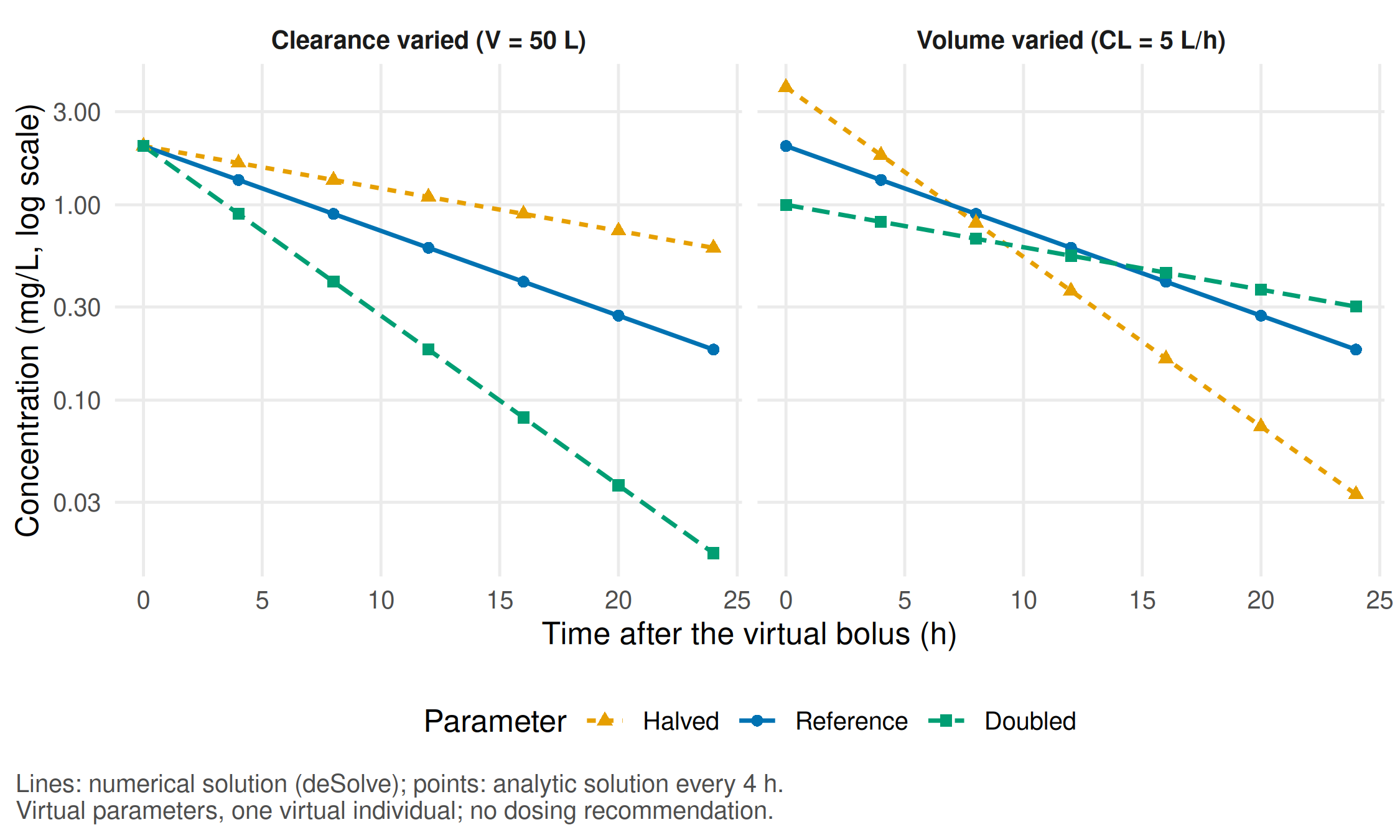
Report. The solver agrees with the analytic solution to a relative difference of 1.5e-10, well inside the tolerance fixed in advance. The half-life is 6.93 h (\(\ln 2 \cdot V / CL\)). Changing clearance alters only the slope; changing the volume alters the starting concentration and the slope. Samples taken only late after the bolus show the slope, i.e. the ratio CL/V; an early sample is needed to separate the two parameters.
TipCounter-check: predict first
Clearance and volume are both doubled (10 L/h and 100 L). What happens to the half-life, and what happens to the concentration at time zero? Would two samples at 12 and 24 hours tell you that anything changed?
# Counter-check: double clearance AND volume. What happens to half-life and to C(0)?
double_both <- c(CL = 10, V = 100)
c(half_life_h = log(2) * double_both[["V"]] / double_both[["CL"]], c0_mg_per_l = dose / double_both[["V"]])
#> half_life_h c0_mg_per_l
#> 6.931472 1.000000stopifnot(isTRUE(all.equal(log(2) * 100 / 10, half_life)), dose / 100 == 1)
NoteOther implementation: Julia/SciML
DifferentialEquations.jl in Julia (Rackauckas and Nie 2017) offers a wide choice of solvers and built-in tools for parameter sensitivity; it is useful when solver choice itself becomes the question, for example in stiff multi-compartment models. For existing Python pipelines, SciPy solve_ivp (Virtanen et al. 2020) is the direct counterpart of the deSolve call used here. A fair comparison needs identical parameters, units, initial amount and time points, the analytic solution as common reference and the same relative tolerance fixed in advance. Status: conceptual comparison, not run. A statement about speed would need a separate benchmark.
Station operating capacity · Does a third theatre change waiting times?
Decision. The emergency plan of a fictitious hospital asks whether a third operating theatre should be opened during a mass casualty incident (MCI).
Assumption. Twelve casualties need surgery; they arrive on average every 15 minutes, and an operation lasts on average 90 minutes (log-normal, assumption). Theatres work first come, first served, without triage priorities. The model describes this scenario only; it is not a prediction for a real incident. Both capacity scenarios are run on the same 200 pre-generated sequences of arrival and operating times (common random numbers), so that any difference comes from capacity and not from chance.
# Part B, station mass casualty incident (unit 22): 12 casualties who need surgery,
# two capacity scenarios on the SAME pre-generated arrival and operating times (common random numbers)
set.seed(20260322)
n_rep <- 200
n_casualties <- 12
mci_events <- do.call(rbind, lapply(seq_len(n_rep), function(r) {
  data.frame(replication = r, casualty = seq_len(n_casualties),
             arrival_min = round(cumsum(rexp(n_casualties, rate = 1 / 15)), 2),          # mean gap 15 min
             surgery_min = round(rlnorm(n_casualties, log(90) - 0.35^2 / 2, 0.35), 2))  # mean 90 min
}))
head(mci_events, 4)
#> replication casualty arrival_min surgery_min
#> 1 1 1 17.44 277.22
#> 2 1 2 34.11 96.26
#> 3 1 3 104.82 83.52
#> 4 1 4 119.69 44.25The queue is written out in a few lines of base R so that every step can be followed. One replication is then re-run in the discrete-event package simmer (Ucar et al. 2019); both must give identical waiting times. The last check confirms that, on identical event sequences, the extra theatre never makes any casualty wait longer.
# Transparent first-come-first-served queue: each casualty takes the theatre that becomes free first
fifo_wait <- function(arrival, surgery, theatres) {
  free_at <- rep(0, theatres)
  start <- numeric(length(arrival))
  for (i in seq_along(arrival)) {
    k <- which.min(free_at)
    start[i] <- max(arrival[i], free_at[k])
    free_at[k] <- start[i] + surgery[i]
  }
  start - arrival                                    # waiting time in minutes
}
mci_events$wait_2 <- NA_real_
mci_events$wait_3 <- NA_real_
for (r in seq_len(n_rep)) {
  rows <- mci_events$replication == r
  mci_events$wait_2[rows] <- fifo_wait(mci_events$arrival_min[rows], mci_events$surgery_min[rows], 2)
  mci_events$wait_3[rows] <- fifo_wait(mci_events$arrival_min[rows], mci_events$surgery_min[rows], 3)
}

# Cross-check with simmer for replication 1: the same events must give the same waiting times
simmer_wait <- function(ev, theatres) {
  casualty <- trajectory("casualty") |>
    seize("theatre", 1) |>
    timeout_from_attribute("surgery_min") |>
    release("theatre", 1)
  env <- simmer("mci") |>
    add_resource("theatre", capacity = theatres) |>
    add_dataframe("casualty", casualty, data = data.frame(time = ev$arrival_min, surgery_min = ev$surgery_min),
                  time = "absolute") |>
    run()
  arr <- get_mon_arrivals(env)
  arr <- arr[order(as.integer(sub("casualty", "", arr$name))), ]
  arr$end_time - arr$start_time - arr$activity_time
}
rep1 <- mci_events[mci_events$replication == 1, ]
check_simmer <- c(two_theatres   = max(abs(simmer_wait(rep1, 2) - rep1$wait_2)),
                  three_theatres = max(abs(simmer_wait(rep1, 3) - rep1$wait_3)))
check_simmer
#> two_theatres three_theatres
#> 5.684342e-14 5.684342e-14stopifnot(all(check_simmer < 1e-8),
all(mci_events$wait_3 <= mci_events$wait_2 + 1e-9)) # more capacity never lengthens a wait hereper_rep <- do.call(rbind, lapply(split(mci_events, mci_events$replication), function(d)
data.frame(replication = d$replication[1],
mean_wait_2_h = mean(d$wait_2) / 60, mean_wait_3_h = mean(d$wait_3) / 60,
over_2h_2 = mean(d$wait_2 > 120), over_2h_3 = mean(d$wait_3 > 120))))
per_rep$difference_h <- per_rep$mean_wait_2_h - per_rep$mean_wait_3_h
spread <- function(x) sprintf("%.2f (%.2f to %.2f)", median(x), quantile(x, 0.1), quantile(x, 0.9))
mci_summary <- data.frame(
measure = c("Mean waiting time per casualty (h)", "Share of casualties waiting > 2 h"),
two_theatres = c(spread(per_rep$mean_wait_2_h), spread(per_rep$over_2h_2)),
three_theatres = c(spread(per_rep$mean_wait_3_h), spread(per_rep$over_2h_3)),
paired_difference = c(spread(per_rep$difference_h), spread(per_rep$over_2h_2 - per_rep$over_2h_3))
)
print(mci_summary, row.names = FALSE)#> measure two_theatres three_theatres
#> Mean waiting time per casualty (h) 2.45 (1.72 to 3.32) 1.08 (0.57 to 1.68)
#> Share of casualties waiting > 2 h 0.58 (0.42 to 0.67) 0.17 (0.00 to 0.42)
#> paired_difference
#> 1.37 (1.07 to 1.64)
#> 0.33 (0.17 to 0.58)stopifnot(nrow(per_rep) == n_rep, all(per_rep$difference_h >= 0))mci_long <- data.frame(
scenario = factor(rep(c("2 operating theatres", "3 operating theatres"), each = n_rep),
levels = c("2 operating theatres", "3 operating theatres")),
mean_wait_h = c(per_rep$mean_wait_2_h, per_rep$mean_wait_3_h)
)
p_mci <- ggplot(mci_long, aes(scenario, mean_wait_h, colour = scenario, shape = scenario)) +
geom_jitter(width = 0.15, height = 0, alpha = 0.5, size = 1.4) +
geom_boxplot(fill = NA, colour = "grey20", outlier.shape = NA, width = 0.45) +
scale_colour_manual(values = unname(cdsr_colours[c("red", "blue")]), guide = "none") +
scale_shape_manual(values = cdsr_shapes[1:2], guide = "none") +
labs(x = NULL, y = "Mean waiting time for surgery per casualty (h)",
caption = paste("Each point is one simulated incident with 12 casualties; n = 200 replications per scenario,",
"both scenarios on identical event sequences. Synthetic.", sep = "\n")) +
theme_cdsr()
show_figure(p_mci, "w6-mci.png")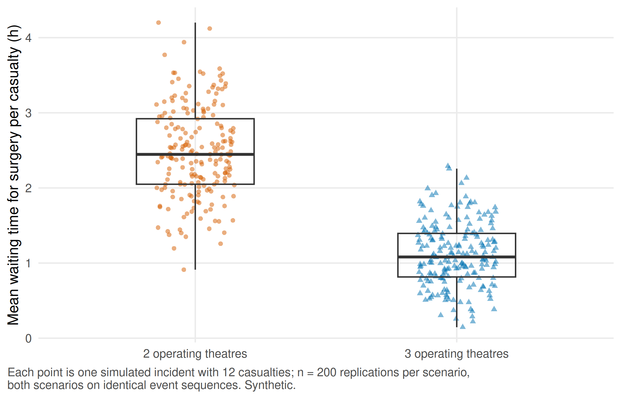
Report. In this scenario the median of the mean waiting time per casualty falls from 2.45 h with two theatres to 1.08 h with three; the paired difference is 1.37 (1.07 to 1.64) h (median and 10th to 90th percentile over 200 replications). The spread over replications belongs in the report: it shows how much a single incident can deviate from the median. Whether the third theatre can be staffed at all, and who waits under triage rules, are questions this model does not answer.
TipCounter-check: predict first
Operations take 20% longer than assumed, while arrivals stay the same. With three theatres, will the median waiting time end up closer to the original three-theatre value or to the two-theatre value?
# Counter-check: operations take 20% longer (same arrivals). How much of the third theatre's gain remains?
longer_3 <- sapply(split(mci_events, mci_events$replication), function(d)
  mean(fifo_wait(d$arrival_min, 1.2 * d$surgery_min, 3)) / 60)
c(median_3_theatres_h = median(per_rep$mean_wait_3_h), median_3_theatres_longer_h = median(longer_3),
  median_2_theatres_h = median(per_rep$mean_wait_2_h))
#> median_3_theatres_h median_3_theatres_longer_h
#> 1.081285 1.518463
#> median_2_theatres_h
#> 2.446785stopifnot(median(longer_3) > median(per_rep$mean_wait_3_h), median(longer_3) < median(per_rep$mean_wait_2_h))
NoteOther implementation: Python/SimPy
SimPy describes each casualty as a Python process; interruptions, priorities and shared staff can be traced line by line, which helps when the plan grows beyond a single queue. The R counterpart is simmer. For a fair comparison, both programs read the same file of arrival and operating times (w6-mci-events.csv); first compare the order of events for one replication, then the waiting times. The same seed number in R and Python does not produce the same random draws, so random numbers are never generated separately in each language. Status: conceptual comparison, not run.
Part C · Three events in twelve animals (unit 23)
Decision. A fictitious preclinical group observed an adverse event (for example a wound infection) in 3 of 12 animals after a new implant. Before planning another experiment, the group wants to state what this result says about the event probability, and what it cannot say.
Assumption. The animals are independent and share one event probability. Two plausible priors are compared: a flat prior Beta(1, 1), and a sceptical prior Beta(2, 8) that expects about 20% events from earlier, similar work (assumption). With a binomial result the posterior is again a Beta distribution, so no sampling algorithm is needed: the 95% intervals come straight from qbeta(). A grid calculation checks the result independently.
# Part C (unit 23): 3 of 12 fictitious animals show the event; two plausible priors
events  <- 3
animals <- 12
priors <- data.frame(prior = c("Flat prior Beta(1, 1)", "Sceptical prior Beta(2, 8)"), a = c(1, 2), b = c(1, 8))
priors$a_post <- priors$a + events
priors$b_post <- priors$b + animals - events
priors$post_mean <- priors$a_post / (priors$a_post + priors$b_post)
priors$lower_95  <- qbeta(0.025, priors$a_post, priors$b_post)
priors$upper_95  <- qbeta(0.975, priors$a_post, priors$b_post)
print(priors, digits = 3)
#> prior a b a_post b_post post_mean lower_95 upper_95
#> 1 Flat prior Beta(1, 1) 1 1 4 10 0.286 0.0909 0.538
#> 2 Sceptical prior Beta(2, 8) 2 8 5 17 0.227 0.0822 0.419# Independent numerical check: posterior on a grid (prior x likelihood) gives the same quantiles
grid <- seq(0, 1, length.out = 200001)
grid_quantiles <- t(sapply(seq_len(nrow(priors)), function(i) {
post <- dbeta(grid, priors$a[i], priors$b[i]) * dbinom(events, animals, grid)
cdf <- cumsum(post) / sum(post)
c(grid[which(cdf >= 0.025)[1]], grid[which(cdf >= 0.975)[1]])
}))
stopifnot(
all(priors$a_post == c(4, 5)), all(priors$b_post == c(10, 17)),
max(abs(grid_quantiles - cbind(priors$lower_95, priors$upper_95))) < 1e-3
)dens <- do.call(rbind, lapply(seq_len(nrow(priors)), function(i) {
p <- seq(0, 1, by = 0.002)
rbind(data.frame(prior = priors$prior[i], curve = "Prior", p = p, density = dbeta(p, priors$a[i], priors$b[i])),
data.frame(prior = priors$prior[i], curve = "Posterior", p = p,
density = dbeta(p, priors$a_post[i], priors$b_post[i])))
}))
dens$curve <- factor(dens$curve, levels = c("Prior", "Posterior"))
p_post <- ggplot(dens, aes(p, density, colour = curve, linetype = curve)) +
geom_vline(xintercept = events / animals, colour = cdsr_colours[["orange"]], linewidth = 0.5) +
geom_line(linewidth = 0.8) +
facet_wrap(~ prior) +
scale_colour_manual(values = unname(cdsr_colours[c("grey", "blue")])) +
scale_linetype_manual(values = cdsr_linetypes[c(2, 1)]) +
scale_x_continuous(labels = scales::percent, name = "Event probability per animal") +
labs(y = "Density", colour = NULL, linetype = NULL,
caption = "Orange line: observed 3 of 12 fictitious animals (25%); n = 12 animals, no control group. Synthetic.") +
theme_cdsr()
show_figure(p_post, "w6-posterior.png", width = 7.5)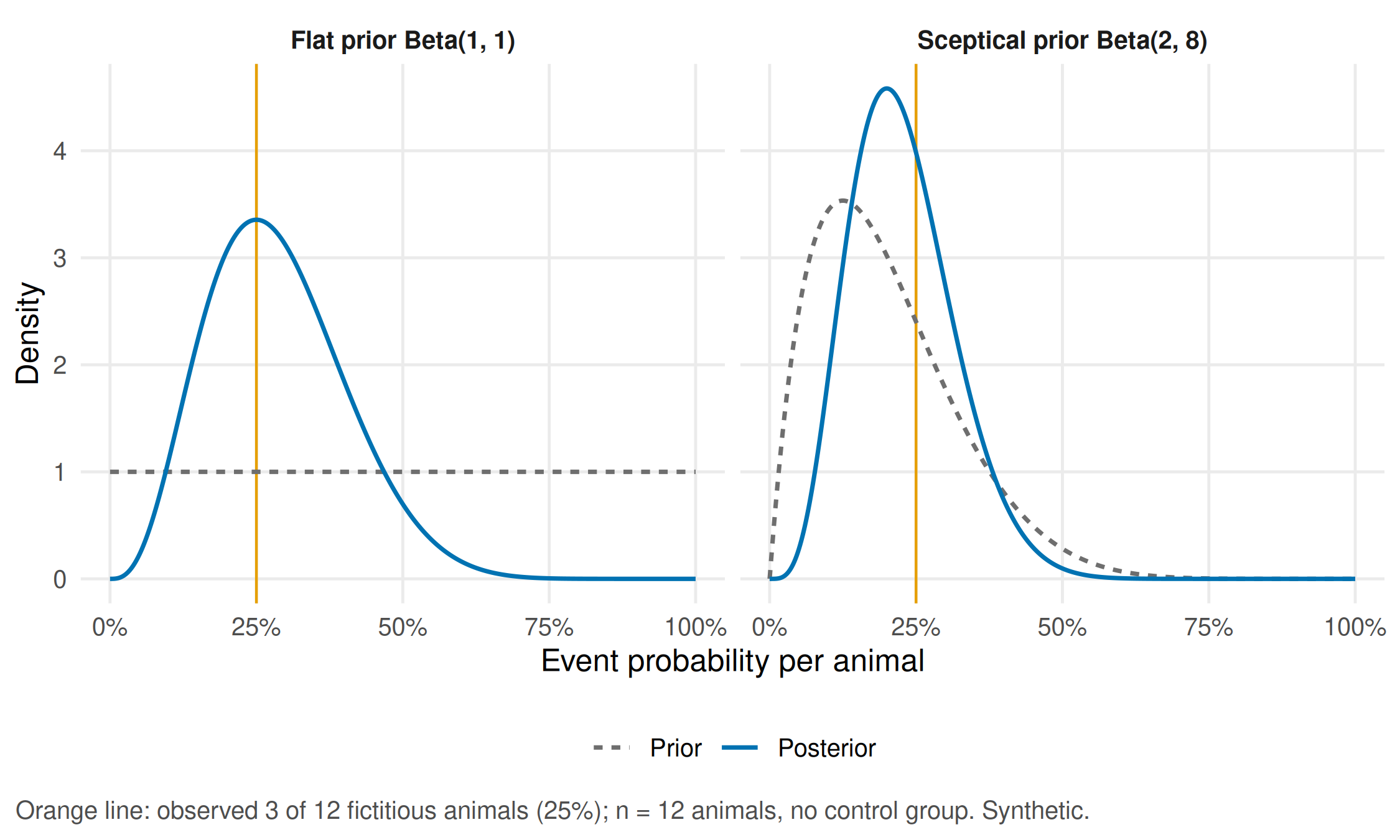
Report. “In 12 animals, 3 had the event. With a flat prior, an event probability between 9.1% and 53.8% is compatible with this result (95% interval); with a sceptical prior based on earlier work, between 8.2% and 41.9%. Without a control group, we cannot say whether the implant caused any of the events.” The event rate describes what happened in these animals; a treatment effect would need a comparison group under the same conditions.
TipCounter-check: predict first
The same rate is observed in ten times as many animals (30 of 120). Will the two intervals become narrower, and will the choice of prior matter more or less?
# Counter-check: the same rate, ten times more animals (30 of 120). Narrower intervals, closer priors?
big <- data.frame(prior = priors$prior, a_post = priors$a + 30, b_post = priors$b + 90)
big$lower_95 <- qbeta(0.025, big$a_post, big$b_post)
big$upper_95 <- qbeta(0.975, big$a_post, big$b_post)
print(big, digits = 3)
#> prior a_post b_post lower_95 upper_95
#> 1 Flat prior Beta(1, 1) 31 91 0.181 0.335
#> 2 Sceptical prior Beta(2, 8) 32 98 0.176 0.323stopifnot(all(big$upper_95 - big$lower_95 < priors$upper_95 - priors$lower_95))
WarningCommon mistake
Reading the posterior as evidence that the implant is harmful or safe. Without a concurrent control group, the posterior describes the event probability under this protocol, not a treatment effect. Whether a further experiment is justified is a 3Rs decision (replacement, reduction, refinement): the next study should answer a question that this result cannot.
Unit 24 · Project workshop: reproduce one number
Run your group’s model against its baseline and its counter-check. Then hand your script to another group. That group starts a fresh R session (for this lab: Rscript r/w6-forecast-pk-simulation.R from the repository root) and reproduces exactly one number that you name in advance, for example the half-life of 6.93 h or the MAE of the 4-week mean before the wave (1.83). If the number differs, record why: missing file, different seed, different package version or a step that was only done by hand.
Your record for the workshop
- Part A: the error table with horizon, MAE, interval coverage and the shift with the largest under-forecast, plus one sentence for the nurse manager.
- Part B: either the PK curve with units, tolerance and the result of the solver check, or the waiting-time distribution with its spread over replications and the paired difference.
- Part C: both posterior intervals and a plain-language sentence that mentions the missing comparison group.
- Unit 24: the number another group reproduced, and the next test you propose on another cohort, period or species.
Download the tables linked at the top if you want to continue in a spreadsheet; w6-mci-events.csv is also the common input for a comparison with another simulation program. The script writes the same files to output/ when you run it on your own.
Further reading
- Companion book: B17 · Forecasting patient flow (required for W6), and either B15 · Mechanistic models and pharmacometrics or B18 · Mass casualty incidents, operating capacity and simulation, depending on your station; B16 · Bayes, small samples and the 3Rs for Part C.
- Methods in R: Rolling-Origin Cross-Validation and Forecast Accuracy Metrics – how to test forecasts on later periods and which error measure answers which question.
- Forecasting: Principles and Practice by Hyndman and Athanasopoulos – the standard open textbook on seasonal baselines and prediction intervals.
- CTTIR Courses: SIR and SEIR models with deSolve – the same solver applied to a compartment model of infection.
- Strategy in R: Monte Carlo Methods for Games – replications, random seeds and the spread of simulated outcomes.
- Methods in R: The Beta-Binomial Model and CTTIR Tutorials: Prior Specification – conjugate updating and how to justify a prior.