6 Accuracy, calibration and clinical utility
R. Heller · Date: 2025-09-07 · Last changed: 2026-11-14
6.1 Case and decision
The orthogeriatric team from Chapter 5 has chosen the prespecified logistic regression for its pilot. Now the standard operating procedure needs one number: from which predicted risk of postoperative delirium is a patient offered proactive geriatric co-management? The ward manager remembers a slide that said “AUC 0.77” and asks whether that settles it. The orthogeriatrician worries about something else: the oldest patients seem to be flagged almost always, while a 74-year-old with several risk factors was not flagged last month and developed delirium. The team has to fix a threshold, say how many alarms per week it will produce, and explain to the nursing staff which patients will be missed. A threshold that is too low exhausts geriatric capacity; one that is too high leaves preventable delirium unaddressed — and the two errors do not fall on the same patients.
6.2 Core reading
A prediction model produces two kinds of information. It ranks patients from lower to higher risk, and it attaches a number to each patient, the predicted probability. Different measures judge different parts of this output, and a model can be good at one and poor at the other.
Discrimination: does the ranking work? The area under the ROC curve (AUC, also called the c-statistic) is the probability that a randomly chosen patient who develops delirium receives a higher predicted risk than a randomly chosen patient who does not. For our model on the 400 test patients it is 0.77. The AUC uses only the order of the predictions; multiplying every risk by two would not change it (Methods in R: ROC and AUC for Logistic Models). It therefore cannot tell whether a predicted risk of 20% means that about one in five such patients develops delirium, and it does not involve any threshold.
Accuracy at a threshold: what happens to people? Once the team decides to act on predicted risks of 20% or more, every test patient falls into one cell of a 2 × 2 table (Table 6.1). The table is the most direct translation of a model into consequences, and it is clearer in absolute numbers than in percentages (Hoffrage and Gigerenzer 1998). Of 1,000 patients like these, about 258 will develop delirium. At the 20% threshold the model flags about 456. Of the flagged patients, about 188 will develop delirium and about 268 will not. About 70 patients who will develop delirium are not flagged. Sensitivity is 72.8%, the positive predictive value 41.2%.
| At a threshold of 20% | Delirium develops | No delirium | Total |
|---|---|---|---|
| Flagged (risk ≥ 20%) | 75 | 107 | 182 |
| Not flagged | 28 | 190 | 218 |
| Total | 103 | 297 | 400 |
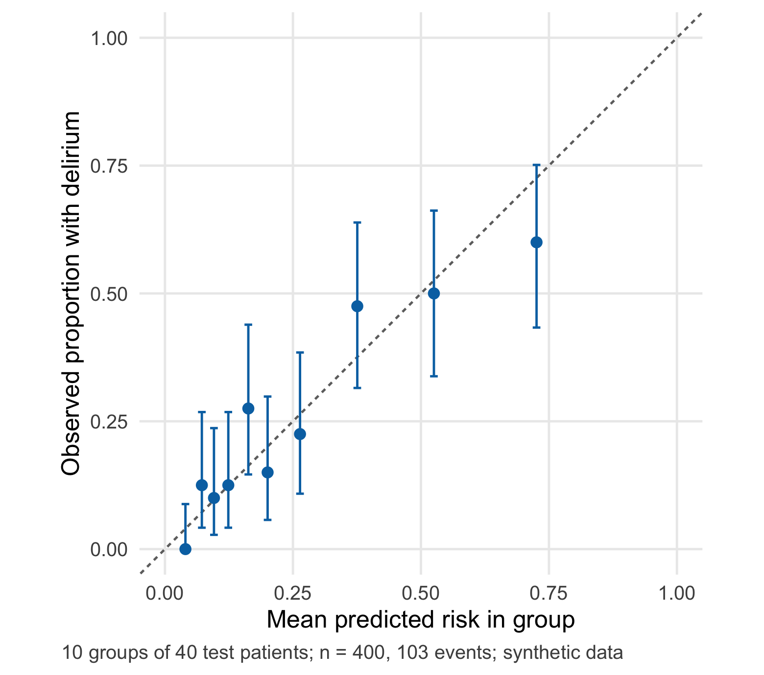
Calibration: can the number be taken at face value? A model is calibrated when, among patients with a predicted risk of about 20%, about 20% develop the outcome. Figure 6.1 groups the test patients into ten groups of 40 by predicted risk and compares the mean prediction with the observed proportion. Points near the diagonal mean that the numbers can be read as risks. Two summaries go with the plot. The calibration intercept (here -0.01) shows whether risks are too high or too low on average; zero is ideal. The calibration slope (here 0.87) shows whether they are too extreme or too timid; one is ideal (Van Calster et al. 2019). Our model is close to the ideal on average, with a slope slightly below 1 — a mild sign of overfitting that the counter-check in Chapter 5 made more visible.
The threshold is a value judgement. Choosing 20% means that the team accepts flagging up to four patients without delirium (80 : 20) for each patient with delirium whom it reaches. This is not a statistical property; it expresses how the team weighs a missed case against an unnecessary consultation. Decision curve analysis makes this explicit by computing the net benefit of the model across thresholds (Vickers and Elkin 2006), and it belongs in every evaluation of a model meant for clinical decisions (Steyerberg et al. 2010). The lab computes it.
Same model, same threshold, two groups. Table 6.2 splits the test patients by age. The model is calibrated in both groups: the mean predicted risk is close to the observed proportion in each. Yet the consequences differ sharply. Among patients aged 80 or older, 74% are flagged and 11 of 78 delirium cases are missed. Among patients aged 65–79, only 22 of 183 are flagged and 17 of 25 delirium cases are missed. The reason is not a faulty model but the lower base rate in the younger group, which places most of its future cases below the threshold.
| Age group | Patients | With delirium | Flagged | Cases found | Cases missed | Flagged without delirium | Mean predicted | Observed |
|---|---|---|---|---|---|---|---|---|
| 65–79 years | 183 | 25 | 22 | 8 | 17 | 14 | 11.9% | 13.7% |
| 80 years or older | 217 | 78 | 160 | 67 | 11 | 93 | 37.6% | 35.9% |
Four measures, four questions. It helps to keep the measures apart by the question each answers. The AUC answers “does the model put patients in the right order?” Calibration answers “can I read the number as a risk?” The 2 × 2 table at a threshold answers “how many patients are flagged, found and missed, and how much work follows?” Net benefit answers “is acting on the model better than treating everybody or nobody, given how we weigh the two errors?” A report that gives only the first answer leaves the clinical team to guess the other three. Overall measures such as the Brier score, the mean squared difference between predicted risk and outcome, combine ranking and calibration in one number and are useful for comparing models, but they do not replace the others (Steyerberg et al. 2010) (Methods in R: Diagnostic Test Accuracy).
The most important assumption of this chapter is that the predicted risks are calibrated in the population and setting where the threshold is applied. A threshold on the probability scale is only meaningful if the probability is right. If the outcome becomes more common, or is recorded more thoroughly, the ranking may stay as good as before while every number is too low — and the threshold quietly stops meaning what the team decided. The counter-check shows this.
Question for the workshop: The 20% threshold flags 46% of patients, more than the 30% capacity of the team. Would you raise the threshold, accept a lower sensitivity in the younger group, or argue for more capacity — and how would you explain your choice to a 74-year-old patient who is not flagged?
6.3 Lab
6.3.1 Step 1 · Read the teaching file and confirm the test patients
The lab reads the cohort written by Chapter 5. A checksum of the sorted test IDs proves that the test patients are the same as there.
cohort <- read.csv("../data/b05-delirium-cohort.csv")
dev <- cohort[cohort$split == "development", ]
test <- cohort[cohort$split == "test", ]
stopifnot(nrow(cohort) == 1200, nrow(test) == 400, sum(test$delirium) == 103,
          length(intersect(dev$id, test$id)) == 0,
          digest::digest(sort(test$id)) == "9b43cfb98549b2a4c17e4feaca07de46")
6.3.2 Step 2 · Refit the prespecified logistic regression
Preprocessing and model are exactly those of Chapter 5: medians from the development data, eight predictors, linear terms.
core <- c("age", "cognitive_impairment", "asa", "haemoglobin", "sodium", "n_medications",
          "hours_to_surgery", "sensory_impairment")
medians <- sapply(dev[core], median, na.rm = TRUE)          # learned on development data only
impute <- function(d) { for (v in core) d[[v]][is.na(d[[v]])] <- medians[[v]]; d }
dev <- impute(dev); test <- impute(test)
fit <- glm(reformulate(core, "delirium"), family = binomial, data = dev)
p <- predict(fit, test, type = "response")                  # predicted risk, test patients
y <- test$delirium                                          # observed outcome, 0/1
auc_test <- local({ r <- rank(p); n1 <- as.double(sum(y)); n0 <- length(y) - n1
  (sum(r[y == 1]) - n1 * (n1 + 1) / 2) / (n1 * n0) })
stopifnot(abs(auc_test - 0.770) < 0.001)                    # identical to B05
per1000 <- function(x) round(1000 * x / length(y))          # natural frequency per 1,000 patients
6.3.3 Step 3 · The 2 × 2 table at a threshold of 20%
threshold <- 0.20
flag <- p >= threshold
tab <- c(tp = sum(flag & y == 1), fp = sum(flag & y == 0),
         fn = sum(!flag & y == 1), tn = sum(!flag & y == 0))
sens <- tab[["tp"]] / sum(y)                     # flagged among patients with delirium
spec <- tab[["tn"]] / sum(1 - y)                 # not flagged among patients without delirium
ppv <- tab[["tp"]] / sum(flag)                   # delirium among flagged patients
npv <- tab[["tn"]] / sum(!flag)                  # no delirium among non-flagged patients
stopifnot(tab[["tp"]] == 75, tab[["fp"]] == 107, tab[["fn"]] == 28, tab[["tn"]] == 190)
exact_ci <- function(x, n) binom.test(x, n)$conf.int   # Clopper-Pearson interval
round(rbind(sensitivity = c(sens, exact_ci(tab[["tp"]], sum(y))),
            specificity = c(spec, exact_ci(tab[["tn"]], sum(1 - y))),
            ppv = c(ppv, exact_ci(tab[["tp"]], sum(flag))),
            npv = c(npv, exact_ci(tab[["tn"]], sum(!flag)))), 3)
#> [,1] [,2] [,3]
#> sensitivity 0.728 0.632 0.811
#> specificity 0.640 0.582 0.694
#> ppv 0.412 0.340 0.487
#> npv 0.872 0.820 0.913The intervals are wide because the denominators are small: 103 patients with delirium for the sensitivity, 182 flagged patients for the positive predictive value. Every percentage in a report should come with its denominator (CTTIR Courses, Course 1 · Diagnostic testing: Se, Sp, PPV, NPV, LR).
6.3.4 Step 4 · AUC with an uncertainty interval
Two common intervals are compared: the analytical DeLong interval (DeLong et al. 1988) as implemented in pROC (Robin et al. 2011), and a percentile bootstrap over patients.
library(pROC)
roc_obj <- roc(y, p, levels = c(0, 1), direction = "<", quiet = TRUE)
ci_delong <- as.numeric(ci.auc(roc_obj, method = "delong"))[c(1, 3)]
set.seed(6062)
boot_auc <- replicate(2000, {
  i <- sample(length(y), replace = TRUE)
  as.numeric(auc(roc(y[i], p[i], levels = c(0, 1), direction = "<", quiet = TRUE)))
})
ci_boot <- quantile(boot_auc, c(0.025, 0.975))
stopifnot(abs(as.numeric(auc(roc_obj)) - auc_test) < 1e-12)
round(rbind(DeLong = ci_delong, bootstrap = ci_boot), 3)
#> 2.5% 97.5%
#> DeLong 0.718 0.822
#> bootstrap 0.718 0.820Both intervals run from about 0.72 to 0.82. With 103 events, a second model would need a clearly larger AUC before any difference could be claimed — one reason why Chapter 5 did not crown a winner.
6.3.5 Step 5 · Calibration: plot, intercept and slope
lp <- qlogis(p)                                             # linear predictor (log-odds)
cal_int <- unname(coef(glm(y ~ offset(lp), family = binomial))[1])   # calibration-in-the-large
cal_slope <- unname(coef(glm(y ~ lp, family = binomial))[2])         # calibration slope
o_e <- sum(y) / sum(p)                                      # observed / expected events
bins <- cut(rank(p, ties.method = "first"), 10, labels = FALSE)      # ten groups of 40
cal <- do.call(rbind, lapply(split(seq_along(p), bins), function(i) {
  ci <- binom.test(sum(y[i]), length(i))$conf.int
  data.frame(n = length(i), predicted = mean(p[i]), observed = mean(y[i]),
             lower = ci[1], upper = ci[2])
}))
stopifnot(all(cal$n == 40), abs(cal_int) < 0.05, cal_slope > 0.8, cal_slope < 0.95)
round(c(intercept = cal_int, slope = cal_slope, observed_expected = o_e), 3)
#> intercept slope observed_expected
#> -0.007 0.865 0.996The following code draws Figure 6.1 in the core reading.
library(ggplot2)
ggplot(cal, aes(x = predicted, y = observed)) +
  geom_abline(intercept = 0, slope = 1, linetype = cdsr_linetypes[2], colour = cdsr_colours[["grey"]]) +
  geom_errorbar(aes(ymin = lower, ymax = upper), width = 0.015, colour = cdsr_colours[["blue"]]) +
  geom_point(size = 2.4, shape = cdsr_shapes[1], colour = cdsr_colours[["blue"]]) +
  coord_equal(xlim = c(0, 1), ylim = c(0, 1)) +
  labs(x = "Mean predicted risk in group", y = "Observed proportion with delirium",
       caption = "10 groups of 40 test patients; n = 400, 103 events; synthetic data") +
  theme_cdsr()
A smooth calibration curve is an alternative to grouped points but needs larger samples to be stable (Van Calster et al. 2019); with 400 patients the grouped version with intervals is the more honest display (Methods in R: Calibration Plots).
6.3.6 Step 6 · From one threshold to many
at_threshold <- function(t) {
  f <- p >= t
  c(threshold = t, flagged = sum(f), flagged_pct = mean(f), tp = sum(f & y == 1),
    fp = sum(f & y == 0), fn = sum(!f & y == 1), sensitivity = sum(f & y == 1) / sum(y),
    ppv = sum(f & y == 1) / sum(f), alarms_per_case = sum(f) / sum(f & y == 1))
}
thr <- as.data.frame(t(sapply(c(0.10, 0.15, 0.20, 0.30, 0.40), at_threshold)))
stopifnot(thr$flagged[thr$threshold == 0.30] <= 0.32 * length(y))   # 30% threshold fits the capacity
knitr::kable(thr, digits = c(2, 0, 2, 0, 0, 0, 2, 2, 1), row.names = FALSE,
             col.names = c("Threshold", "Flagged", "Share flagged", "Cases found", "Flagged, no delirium",
                           "Cases missed", "Sensitivity", "PPV", "Alarms per case found"),
caption = "Consequences of five thresholds for the same model on 400 synthetic test patients (103 with delirium).")| Threshold | Flagged | Share flagged | Cases found | Flagged, no delirium | Cases missed | Sensitivity | PPV | Alarms per case found |
|---|---|---|---|---|---|---|---|---|
| 0.10 | 292 | 0.73 | 96 | 196 | 7 | 0.93 | 0.33 | 3.0 |
| 0.15 | 235 | 0.59 | 88 | 147 | 15 | 0.85 | 0.37 | 2.7 |
| 0.20 | 182 | 0.46 | 75 | 107 | 28 | 0.73 | 0.41 | 2.4 |
| 0.30 | 126 | 0.32 | 65 | 61 | 38 | 0.63 | 0.52 | 1.9 |
| 0.40 | 92 | 0.23 | 50 | 42 | 53 | 0.49 | 0.54 | 1.8 |
The last column is the number of flagged patients per delirium case reached, the reciprocal of the positive predictive value. Of the five thresholds, 30% is the lowest that keeps the share of flagged patients near the team’s capacity of about 30%; it does so at the price of 38 missed cases instead of 28.
6.3.7 Step 7 · Net benefit and the decision curve
Net benefit counts correctly flagged patients and subtracts flagged patients without delirium, weighted by the odds of the threshold: NB = TP/n − FP/n × t/(1 − t) (Vickers and Elkin 2006). It is compared with flagging everybody and flagging nobody (net benefit 0).
ts <- seq(0.05, 0.50, by = 0.01)
nb_model <- sapply(ts, function(t) { f <- p >= t
  sum(f & y == 1) / length(y) - sum(f & y == 0) / length(y) * t / (1 - t) })
prev <- mean(y)
nb_all <- prev - (1 - prev) * ts / (1 - ts)
dca <- rbind(data.frame(threshold = ts, net_benefit = nb_model, strategy = "Model"),
             data.frame(threshold = ts, net_benefit = nb_all, strategy = "Flag everybody"),
             data.frame(threshold = ts, net_benefit = 0, strategy = "Flag nobody"))
nb20 <- nb_model[which.min(abs(ts - 0.20))]
stopifnot(nb20 > nb_all[which.min(abs(ts - 0.20))], nb20 > 0)library(ggplot2)
ggplot(dca, aes(x = threshold, y = net_benefit, colour = strategy, linetype = strategy)) +
geom_line(linewidth = 0.9) +
geom_vline(xintercept = 0.20, colour = cdsr_colours[["grey"]], linetype = cdsr_linetypes[4]) +
scale_colour_manual(values = c(Model = cdsr_colours[["blue"]], `Flag everybody` = cdsr_colours[["orange"]],
`Flag nobody` = cdsr_colours[["grey"]])) +
scale_linetype_manual(values = c(Model = cdsr_linetypes[1], `Flag everybody` = cdsr_linetypes[2],
`Flag nobody` = cdsr_linetypes[3])) +
coord_cartesian(ylim = c(-0.05, 0.27)) +
labs(x = "Threshold probability", y = "Net benefit", colour = NULL, linetype = NULL,
caption = "Vertical line: threshold of 20%. n = 400 test patients; synthetic data") +
theme_cdsr()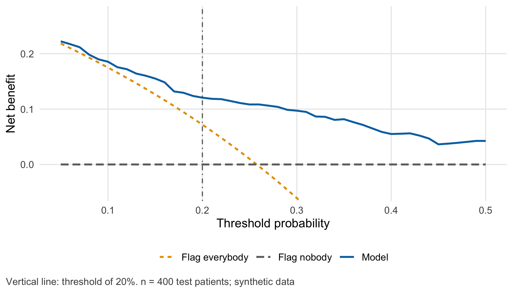
At 20% the model’s net benefit is 0.121: the equivalent of 121 correctly flagged patients per 1,000 with no unnecessary consultations at all. Decision curves and related measures are practised in CTTIR Courses, Course 2 · Decision curves, NRI, IDI.
6.3.8 Step 8 · Two groups, with denominators
age_group <- ifelse(test$age >= 80, "80+", "65-79")
grp <- t(sapply(c("65-79", "80+"), function(g) {
  i <- age_group == g
  c(n = sum(i), cases = sum(y[i]), alarms = sum(flag[i]), tp = sum(flag[i] & y[i] == 1),
    fn = sum(!flag[i] & y[i] == 1), fp = sum(flag[i] & y[i] == 0),
    mean_pred = mean(p[i]), observed = mean(y[i]))
}))
sens_ci <- t(sapply(rownames(grp), function(g) exact_ci(grp[g, "tp"], grp[g, "cases"])))
stopifnot(sum(grp[, "n"]) == 400, sum(grp[, "tp"]) == tab[["tp"]], sum(grp[, "fn"]) == tab[["fn"]],
          grp["65-79", "fn"] == 17, grp["80+", "fn"] == 11)
round(cbind(sensitivity = grp[, "tp"] / grp[, "cases"], lower = sens_ci[, 1], upper = sens_ci[, 2]), 2)
#> sensitivity lower upper
#> 65-79 0.32 0.15 0.54
#> 80+ 0.86 0.76 0.93In the younger group the sensitivity is 32% with an interval from 15% to 54%, based on only 25 cases. The difference to the older group is large, but the younger group’s estimate is imprecise. TRIPOD+AI asks for performance estimates with confidence intervals, including for key subgroups (Collins et al. 2024, item 23a).
6.4 Counter-check
Change one assumption: how delirium is recorded. Suppose that the ward introduces a structured delirium screen twice a day instead of relying on notes. More mild episodes are recorded. We represent this as an assumption: the log-odds of recorded delirium rise by 0.8 for every patient, while the patients and their predictors stay the same. Because the data are synthetic, each patient’s true risk is known and the new outcomes can be simulated.
Before you run the code, predict: Does the AUC fall, stay or rise? Does the calibration intercept move, and in which direction? How many patients whose (new) risk is at least 20% will the unchanged 20% threshold miss?
set.seed(6061)
risk_b <- plogis(qlogis(test$true_risk) + 0.8)              # true risk under the new recording (assumption)
y_b <- rbinom(length(risk_b), 1, risk_b)                    # recorded delirium, setting B
auc_b <- as.numeric(auc(roc(y_b, p, levels = c(0, 1), direction = "<", quiet = TRUE)))
cal_int_b <- unname(coef(glm(y_b ~ offset(lp), family = binomial))[1])
missed_high_a <- sum(test$true_risk >= threshold & !flag)   # true risk >= 20%, not flagged, setting A
missed_high_b <- sum(risk_b >= threshold & !flag)           # same, setting B
sens_b <- sum(flag & y_b == 1) / sum(y_b)

# Intercept update: estimate the shift on 200 patients, check it on the other 200
half <- seq_along(p) <= 200
shift <- unname(coef(glm(y_b[half] ~ offset(lp[half]), family = binomial))[1])
p_upd <- plogis(lp + shift)
cal_int_upd <- unname(coef(glm(y_b[!half] ~ offset(qlogis(p_upd[!half])), family = binomial))[1])
stopifnot(abs(auc_b - auc_test) < 0.05, cal_int_b > 0.5, missed_high_b > 3 * missed_high_a,
          abs(cal_int_upd) < abs(cal_int_b))
knitr::kable(data.frame(
  quantity = c("Recorded delirium", "AUC", "Calibration intercept", "Sensitivity at 20%",
               "Patients with true risk ≥ 20% not flagged"),
  setting_a = c(paste0(sum(y), "/400"), sprintf("%.2f", auc_test), sprintf("%.2f", cal_int),
                cdsr_percent(sens), paste0(missed_high_a, " of ", sum(test$true_risk >= threshold))),
  setting_b = c(paste0(sum(y_b), "/400"), sprintf("%.2f", auc_b), sprintf("%.2f", cal_int_b),
                cdsr_percent(sens_b), paste0(missed_high_b, " of ", sum(risk_b >= threshold)))),
  col.names = c("Quantity", "Setting A (as developed)", "Setting B (structured screen)"),
caption = "Counter-check: same model, same 400 synthetic patients, outcome recorded more thoroughly (assumption: +0.8 on the log-odds scale).")| Quantity | Setting A (as developed) | Setting B (structured screen) |
|---|---|---|
| Recorded delirium | 103/400 | 154/400 |
| AUC | 0.77 | 0.79 |
| Calibration intercept | -0.01 | 0.77 |
| Sensitivity at 20% | 72.8% | 70.8% |
| Patients with true risk ≥ 20% not flagged | 31 of 194 | 128 of 310 |
The ranking survives: the AUC is 0.79 instead of 0.77. The numbers do not. The calibration intercept of 0.77 means that the model systematically underestimates risk in setting B, and 128 patients whose risk now exceeds the 20% that the team agreed on are not flagged — compared with 31 in setting A. A team that monitored only the AUC would notice nothing. Updating the intercept on 200 patients from the new setting and checking it on the other 200 reduces the calibration intercept to -0.19. TRIPOD+AI asks authors to describe such model updating and to report the updated model (Collins et al. 2024, items 12f and 24). A different hospital with a higher baseline risk would produce the same pattern; Chapter 19 and Chapter 20 take this further.
6.5 Consequences for patients and operations
Patients and fairness. The age-group table is the core ethical finding of this chapter. With a single threshold, patients aged 65–79 who will develop delirium are missed far more often than older patients, although the model is calibrated in both groups. Lowering the threshold for the younger group would find more of their cases at the cost of more consultations without delirium; it is a value decision that should be made openly, with the affected clinicians and, where possible, patient representatives, and not hidden in code (Chapter 21; Strategy in R: Fairness in Machine Learning). A patient who is not flagged must still receive the usual clinical attention; the threshold allocates an additional offer, it does not withdraw care.
Operations. If about eight eligible patients are admitted per week (assumption), the 20% threshold produces about 3.6 alarms per week and the 30% threshold about 2.5. The procedure should state the threshold, the expected alarms per week, the expected missed cases per 100 patients and the person who reviews these numbers each month. Because calibration can drift unnoticed, monitoring must include observed versus predicted events, not only alarms and AUC (Chapter 20).
Regulation and documentation. The threshold is part of how the software is used. If a manufacturer’s documentation specifies performance at a particular threshold, a local change of threshold changes the conditions under which that claim was made; who may change it, and how this is documented, is a question for the intended purpose and quality management (Chapter 22, open for the local setting).
Data protection. The analyses here use aggregated test results. Subgroup tables with very small cells can make individuals identifiable when published; the rules in Chapter 26 apply before such tables leave the team.
6.6 Look up and transfer
Reviewer question: “Do the authors report calibration (plot, intercept and slope) in the population where the model is meant to be used, and do they translate their chosen threshold into absolute numbers of flagged, found and missed patients — with denominators and intervals for key subgroups?” TRIPOD+AI asks for the measures and plots used to evaluate discrimination, calibration and clinical utility, and for subgroup estimates with confidence intervals (Collins et al. 2024, items 12e and 23a).
Self-test: A colleague reports that a delirium model “performs well” in a rehabilitation clinic: AUC 0.80. In this clinic delirium occurs in 8% of patients, but the mean predicted risk is 24%. The clinic plans to use a 20% threshold. What do you expect for the number of alarms and the positive predictive value, and what would you ask for before the threshold is adopted?
TipAnswer
The model overestimates risk by a factor of about three on average (calibration-in-the-large is poor), so a 20% threshold on these inflated numbers will flag many patients whose true risk is far below 20%. Expect a high share of flagged patients and a low positive predictive value — at an 8% base rate, most alarms will concern patients without delirium. The AUC of 0.80 does not contradict this, because it ignores the absolute level of the predictions. Before adoption, ask for a calibration plot with intercept and slope in this clinic, a recalibration (at least of the intercept) on local data, and a table of flagged, found and missed patients per 100 at the proposed threshold.
Annotated sources:
- Van Calster et al. (2019) explains why poor calibration can make an algorithm misleading for decisions and how to assess calibration at validation.
- Steyerberg et al. (2010) sets out the framework of overall performance, discrimination, calibration and decision-analytic measures used in this chapter.
- Vickers and Elkin (2006) introduces decision curve analysis and the link between threshold probability and the weighing of false-positive and false-negative decisions.
- DeLong et al. (1988) and Robin et al. (2011) are the method and software for the analytical AUC interval in Step 4.
- Hoffrage and Gigerenzer (1998) shows that natural frequencies improve diagnostic reasoning compared with probabilities, supporting the per-1,000 translation.
- Collins et al. (2024) provides the reporting items for performance measures, subgroup estimates and model updating.
6.7 Further reading
- Chapter 5 — how the model, the split and the test patients used here were built.
- Chapter 9 — the same 2 × 2 logic for a diagnostic alert at two different prevalences.
- Chapter 21 — who bears the consequences of missed cases and false alarms, and how to discuss them with patients.
- Methods in R: Week 3, Session 5 — Calibration, discrimination, ROC/AUC, Brier score — a complete lab on the measures of Steps 3 to 5.
- CTTIR Courses, Course 2 · Calibration, discrimination, ROC/AUC, Brier score — the same topic as a course session with exercises.
- CTTIR Courses, Course 4 · Time-dependent Brier, IPA, external validation — performance measures for external validation.
- CTTIR Tutorials: Platt Scaling — recalibration methods beyond the intercept update of the counter-check.
- Methods in R: Cutpoint Selection — why data-driven “optimal” cut-offs need the same caution as data-driven model choice.