| Setting | Tool output | Fracture | No fracture | Total | Share with fracture |
|---|---|---|---|---|---|
| A · 5% prevalence | alert | 45 | 95 | 140 | 45/140 = 32.1% |
| A · 5% prevalence | no alert | 5 | 855 | 860 | 5/860 = 0.6% |
| B · 20% prevalence | alert | 180 | 80 | 260 | 180/260 = 69.2% |
| B · 20% prevalence | no alert | 20 | 720 | 740 | 20/740 = 2.7% |
9 A fracture alert in the emergency department
R. Heller · Date: 2026-07-26 · Last changed: 2026-11-09
9.1 Case and decision
It is the middle of a night shift in a fictitious emergency department. A junior doctor has just looked at the wrist radiograph of a 67-year-old patient who fell on an outstretched hand. She sees no fracture. The image-analysis tool that the department is piloting has placed a box over the distal radius with the label “possible fracture – second look recommended”. The information sheet states a sensitivity and specificity of 90% each; in this chapter both values are assumptions. The doctor now has to choose: call the on-call senior to review the image, splint the wrist and book a follow-up radiograph, or discharge the patient with advice. Before she decides, she asks the question this chapter answers: how often is a box like this one right? The answer depends less on the tool than on who comes through the door.
9.2 Core reading
Two settings, one tool. We compare two hypothetical care settings. In setting A, an emergency department radiographs every patient with a limb injury; 5% of the patients examined actually have a fracture. In setting B, patients are referred from a trauma clinic because a clinician already suspects a fracture; here 20% have one. Each setting examines 1,000 patients. For this calculation we give the tool the same sensitivity (the share of fractures that it flags) and the same specificity (the share of patients without fracture that it leaves unflagged) in both settings: 90% each. This is of the same order as pooled estimates from a meta-analysis of AI fracture detection, in which about half of the included studies had a high risk of bias [Kuo et al. (2022); published]. The key assumption is that sensitivity and specificity do not change between the two settings. In practice this assumption often fails, because the mix of injuries, patients and imaging differs between settings. A meta-epidemiological study of 23 diagnostic meta-analyses found that sensitivity or specificity often varied with prevalence; specificity tended to be lower where prevalence was higher [Leeflang et al. (2013); published]. Any real deployment would therefore have to measure both values locally.
Absolute numbers first. Before any percentage, count people. In setting A, 50 of the 1,000 patients have a fracture. The tool flags 45 of them and misses 5. Of the 950 patients without a fracture, the tool flags 95 and leaves 855 unflagged. In setting B, 200 patients have a fracture: 180 are flagged and 20 are missed. Of the 800 without a fracture, 80 are flagged and 720 are not. Counts of this kind, called natural frequencies, are easier to reason with than conditional probabilities (Hoffrage et al. 2000). Table 9.1 shows them as two fourfold tables and Figure 9.1 shows every patient as one symbol.
Then the denominator. The positive predictive value (PPV) answers the junior doctor’s question: of all patients with an alert, how many have a fracture? Its denominator is every patient with an alert, not every patient with a fracture. In setting A, 140 patients receive an alert and 45 of them have a fracture: the PPV is 45/140 = 32.1%. In setting B the same tool gives 180/260 = 69.2%. Nothing about the software has changed; only the patients have. The negative predictive value (NPV) moves in the other direction, from 99.4% in A to 97.3% in B. A missing alert is therefore not an all-clear: in B, 20 of 1,000 patients have a fracture that the tool did not flag. The general relationship between prevalence and predictive values is worked through in Methods in R: Predictive Values and Prevalence and in the CTTIR lab Diagnostic testing: Se, Sp, PPV, NPV, LR (Altman and Bland 1994).
Code
library(ggplot2)
# One row per patient; categories in the order alert/fracture, alert/no fracture, missed, neither
categories <- c("Alert, fracture (true positive)", "Alert, no fracture (false positive)",
                "No alert, fracture (false negative)", "No alert, no fracture (true negative)")
icons <- do.call(rbind, lapply(1:2, function(i) {
  counts <- c(tp[i], fp[i], fn[i], tn[i])
  data.frame(
    setting = sprintf("%s · prevalence %s · PPV %d/%d = %s", names(prev)[i], cdsr_percent(prev[i], 0),
                      tp[i], alerts[i], cdsr_percent(ppv[i])),
    category = factor(rep(categories, times = counts), levels = categories),
    position = 0:(n_examined - 1)
  )
}))
icons$column <- icons$position %% 50
icons$row <- icons$position %/% 50
ggplot(icons, aes(column, -row, colour = category, shape = category, size = category)) +
  geom_point() +
  facet_wrap(~ setting, ncol = 1) +
  scale_colour_manual(values = unname(c(cdsr_colours["blue"], cdsr_colours["red"],
                                        cdsr_colours["orange"], "grey70"))) +
  scale_shape_manual(values = c(16, 15, 17, 1)) +
  scale_size_manual(values = c(1.9, 1.9, 1.9, 0.9)) +
  guides(colour = guide_legend(ncol = 2), shape = guide_legend(ncol = 2), size = guide_legend(ncol = 2)) +
  coord_equal() +
  labs(x = NULL, y = NULL, colour = NULL, shape = NULL, size = NULL,
       caption = "Synthetic data · n = 1,000 patients per setting · sensitivity = specificity = 90% (assumption)") +
  theme_cdsr() +
  theme(axis.text = element_blank(), panel.grid = element_blank())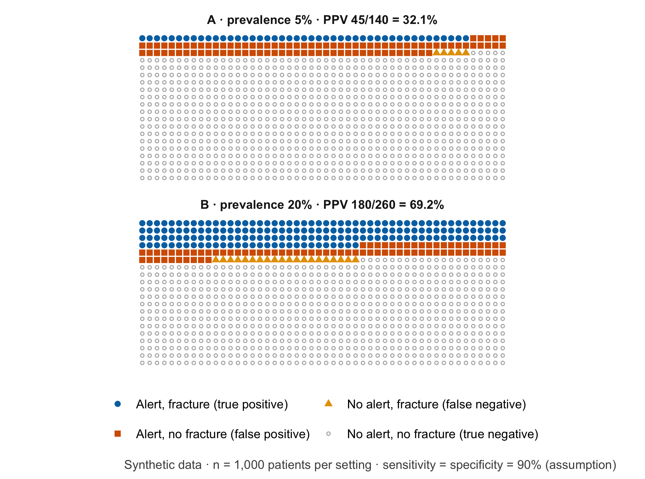
Three research questions, not one. The fourfold table invites a single verdict: “the tool works” or “it does not”. In fact three separate questions are at stake, and each needs its own design.
- Model performance. How well does the tool separate patients with and without fracture, compared with a defined reference standard, in the population where it will be used? This is a diagnostic accuracy study, reported according to STARD-AI (Sounderajah et al. 2025). It yields sensitivity, specificity and predictive values with confidence intervals.
- Patient benefit. Do patients whose images are assessed with the tool have fewer missed fractures with consequences, without more harm from extra imaging, immobilisation or waiting? Accuracy cannot answer this. It needs a comparison group and outcomes that matter to patients, for example in a cluster-randomised or stepped-wedge study.
- Organisational burden. How many additional second looks does the tool create per shift, and who absorbs them? If 1,000 examinations fall into 90 shifts (30 days with three shifts each; an assumption), setting A produces about 1.6 alerts per shift, 1.1 of them false. Setting B produces 2.9 alerts per shift, of which 0.9 are false. Early clinical evaluations of this kind are reported along the lines of DECIDE-AI (Vasey et al. 2022).
Reader study and local pilot answer different questions. In a reader study, several clinicians read the same set of images with and without the tool. Such a study can show whether the tool changes readers’ accuracy under controlled conditions. Its case mix is usually chosen by design: in one multi-reader study of fracture detection on radiographs, the fracture prevalence was fixed at 50% [Guermazi et al. (2022); published]. A PPV from such a set says little about setting A. A local pilot, for example in silent mode, records how often the tool alerts in the department’s own case mix, what the local PPV is and how long second looks take. Neither design on its own shows that patients are better off.
A lower PPV alone is no reason to reject a product. Setting A’s PPV of 32.1% sounds poor. Whether it is acceptable depends on what a false alert costs (a few minutes of a senior clinician’s time, perhaps an extra view) and on what a true alert gains. The gain is not 45 detected fractures: it is the fractures among them that the clinicians would otherwise have missed. Weighing these consequences is a decision analysis, not a property of the PPV (Vickers and Elkin 2006); Chapter 6 develops it with thresholds and net benefit.
Saying it at handover. A spoken handover in setting A could be: “The tool has flagged the distal radius. In a patient group like ours, only about one in three of these flags turns out to be a real fracture, so I would like a second pair of eyes on the image before we decide.” In real operation, the “one in three” has to come from local data, not from this exercise. The patient may then ask: “If the computer is wrong two times out of three, why listen to it at all, and would no box have meant that I could go home?” A good answer explains that the box asks for a second look but does not decide, and that a missing box lowers the probability of a fracture without ruling it out. The clinical findings still count.
Question for the workshop: Your team works in setting A. Which single number would you put on the whiteboard for the night shift – the PPV, the false alerts per shift or the missed fractures per month – and who should be told the other two?
9.3 Lab
The lab recomputes every number from the core reading in base R, from the inputs to the predictive values. In W3, one team works out setting A and another setting B by hand before anyone runs the code. Start a fresh R session in the book folder. The following single line already reproduces both PPVs and is a useful first check that R is running:
# Start command: PPV = true positives / all alerts, for 5% and 20% prevalence
round(100 * 0.9 * c(0.05, 0.20) / (0.9 * c(0.05, 0.20) + 0.1 * c(0.95, 0.80)), 1)
#> [1] 32.1 69.2Step 1 – inputs. Each row describes one setting. Sensitivity and specificity are inputs, not results; in this chapter they are assumptions.
cohorts <- data.frame(
  setting = c("A", "B"),
  description = c("unselected emergency department", "referred with clinical suspicion"),
  examined = c(1000L, 1000L),     # patients examined per setting
  prevalence = c(0.05, 0.20),     # share with fracture according to the reference standard
  sensitivity = c(0.90, 0.90),    # assumption: identical in both settings
  specificity = c(0.90, 0.90)     # assumption: identical in both settings
)
cohorts
#> setting description examined prevalence sensitivity
#> 1 A unselected emergency department 1000 0.05 0.9
#> 2 B referred with clinical suspicion 1000 0.20 0.9
#> specificity
#> 1 0.9
#> 2 0.9Step 2 – absolute frequencies. People are counted in whole numbers, so every count is rounded explicitly.
cohorts$fracture <- round(cohorts$examined * cohorts$prevalence)
cohorts$no_fracture <- cohorts$examined - cohorts$fracture
cohorts$true_pos <- round(cohorts$sensitivity * cohorts$fracture)        # alert and fracture
cohorts$false_neg <- cohorts$fracture - cohorts$true_pos                 # fracture without alert
cohorts$false_pos <- round((1 - cohorts$specificity) * cohorts$no_fracture) # alert without fracture
cohorts$true_neg <- cohorts$no_fracture - cohorts$false_pos              # neither
cohorts[, c("setting", "fracture", "true_pos", "false_neg", "no_fracture", "false_pos", "true_neg")]
#> setting fracture true_pos false_neg no_fracture false_pos true_neg
#> 1 A 50 45 5 950 95 855
#> 2 B 200 180 20 800 80 720Step 3 – denominators and predictive values. The alerts form the denominator of the PPV; the patients without an alert form the denominator of the NPV.
cohorts$alerts <- cohorts$true_pos + cohorts$false_pos
cohorts$no_alerts <- cohorts$false_neg + cohorts$true_neg
cohorts$ppv <- cohorts$true_pos / cohorts$alerts
cohorts$npv <- cohorts$true_neg / cohorts$no_alerts
data.frame(setting = cohorts$setting,
           ppv = paste0(cohorts$true_pos, "/", cohorts$alerts, " = ", cdsr_percent(cohorts$ppv)),
           npv = paste0(cohorts$true_neg, "/", cohorts$no_alerts, " = ", cdsr_percent(cohorts$npv)))
#> setting ppv npv
#> 1 A 45/140 = 32.1% 855/860 = 99.4%
#> 2 B 180/260 = 69.2% 720/740 = 97.3%# Target values from the core reading
stopifnot(
cohorts$true_pos == c(45, 180),
cohorts$false_pos == c(95, 80),
cohorts$alerts == c(140, 260),
isTRUE(all.equal(cohorts$ppv, c(45 / 140, 180 / 260))),
cdsr_percent(cohorts$ppv) == c("32.1%", "69.2%"),
# the lab and the hidden calculation behind the core reading agree
cohorts$true_pos == tp, cohorts$false_pos == fp, cohorts$alerts == alerts
)
WarningCommon mistake
“Sensitivity 90%” is often read as “90% of alerts are right”. Sensitivity is conditioned on the fracture (45 of 50 fractures are flagged); the PPV is conditioned on the alert (45 of 140 alerts are fractures). Swapping the two conditions turns 32.1% into 90% for the same 1,000 patients.
Step 4 – the workload per shift. The number of shifts is an assumption and should be replaced by the local rota. The calculation separates the alerts that need a second look from the false alerts among them.
shifts_per_1000 <- 90  # assumption: 30 days x 3 shifts for 1,000 examinations
cohorts$alerts_per_shift <- cohorts$alerts / shifts_per_1000
cohorts$false_alerts_per_shift <- cohorts$false_pos / shifts_per_1000
cohorts$missed_per_1000 <- cohorts$false_neg
cohorts[, c("setting", "alerts_per_shift", "false_alerts_per_shift", "missed_per_1000")]
#> setting alerts_per_shift false_alerts_per_shift missed_per_1000
#> 1 A 1.555556 1.0555556 5
#> 2 B 2.888889 0.8888889 20stopifnot(round(cohorts$alerts_per_shift, 2) == c(1.56, 2.89))Setting B produces more alerts per shift but fewer false ones: 80 against 95 per 1,000 examinations. Workload and PPV are different quantities, and a team planning staffing needs both.
Step 5 – raw values for download. The fourfold counts are stored as a small table so that W3 groups can start from the file instead of the code.
raw <- cohorts[, c("setting", "description", "examined", "prevalence", "sensitivity", "specificity",
                   "true_pos", "false_pos", "false_neg", "true_neg")]
write.csv(raw, "../data/b09-fracture-alert-cohorts.csv", row.names = FALSE)
# Re-reading the file must give the same PPVs
check <- read.csv("../data/b09-fracture-alert-cohorts.csv")
stopifnot(isTRUE(all.equal(check$true_pos / (check$true_pos + check$false_pos), cohorts$ppv)))
The file data/b09-fracture-alert-cohorts.csv contains only synthetic counts and the two assumptions.
NoteOther implementation: Python with PyTorch
A fracture tool of this kind is usually a convolutional network trained on radiographs. The PyTorch tutorial on transfer learning shows the standard route: start from a ResNet-18 with ImageNet weights (weights='IMAGENET1K_V1'), resize to 256 pixels, crop to 224, normalise with the ImageNet channel means and standard deviations and retrain the final layer (Paszke et al. 2019). The concrete advantage is access to pretrained weights and to research code that already works on images; R would only consume the network’s output. For a fair comparison with the counts in this chapter the following must be identical and written down: the image set and the reference standard, the image orientation (training with random horizontal flips mixes left and right), the conversion of greyscale radiographs to three channels, the weights file and software version (torch 2.15.0 and torchvision 0.29.2 were current in November 2026), and the threshold that turns a probability into an alert. Logit, probability and binary alert should be compared separately. Patients often have two or three views; the counting unit for the fourfold table (patient or image) must be the same on both sides. Status: conceptual comparison, not run.
9.4 Counter-check
Change one assumption and predict the direction before you compute. Suppose the department installs new radiography equipment and the tool’s specificity in setting A drops from 90% to 80%, while sensitivity stays at 90%. Does the PPV halve, fall a little or stay the same? And what happens to the false alerts per shift?
# Function: predictive values and counts for any combination of inputs
fourfold <- function(prevalence, sensitivity, specificity, examined = 1000) {
  fracture <- round(examined * prevalence)
  true_pos <- round(sensitivity * fracture)
  false_pos <- round((1 - specificity) * (examined - fracture))
  data.frame(prevalence, sensitivity, specificity, true_pos, false_pos,
             alerts = true_pos + false_pos, ppv = true_pos / (true_pos + false_pos))
}
changed <- rbind(fourfold(0.05, 0.90, 0.90), fourfold(0.05, 0.90, 0.80))
changed$false_alerts_per_shift <- changed$false_pos / shifts_per_1000
changed
#> prevalence sensitivity specificity true_pos false_pos alerts ppv
#> 1 0.05 0.9 0.9 45 95 140 0.3214286
#> 2 0.05 0.9 0.8 45 190 235 0.1914894
#> false_alerts_per_shift
#> 1 1.055556
#> 2 2.111111stopifnot(changed$false_pos == c(95, 190), round(changed$ppv[2], 3) == 0.191)The false alerts double, from 95 to 190 per 1,000 examinations, while the PPV falls from 32.1% to 19.1%. At low prevalence, specificity drives the workload. Figure 9.2 shows the same reasoning over a range of prevalences.
Code
grid <- expand.grid(prevalence = seq(0.01, 0.40, by = 0.005), specificity = c(0.90, 0.80))
grid$ppv <- 0.90 * grid$prevalence / (0.90 * grid$prevalence + (1 - grid$specificity) * (1 - grid$prevalence))
grid$specificity <- factor(cdsr_percent(grid$specificity, 0), levels = c("90%", "80%"))
marks <- data.frame(prevalence = prev, ppv = ppv, label = paste0(names(prev), ": ", cdsr_percent(ppv)),
                    hjust = c(1.15, -0.15), vjust = c(-0.5, 1.3))  # label A above left, B below right
ggplot(grid, aes(prevalence, ppv, linetype = specificity, colour = specificity)) +
  geom_line(linewidth = 0.9) +
  geom_point(data = marks, aes(prevalence, ppv), inherit.aes = FALSE, size = 2.5) +
  geom_text(data = marks, aes(prevalence, ppv, label = label, hjust = hjust, vjust = vjust),
            inherit.aes = FALSE, size = 3.5) +
  scale_x_continuous(labels = function(x) cdsr_percent(x, 0)) +
  scale_y_continuous(labels = function(x) cdsr_percent(x, 0), limits = c(0, 1)) +
  scale_colour_manual(values = unname(cdsr_colours[c("blue", "red")])) +
  scale_linetype_manual(values = cdsr_linetypes[1:2]) +
  labs(x = "Fracture prevalence (share of patients examined)", y = "Positive predictive value",
       colour = "Specificity", linetype = "Specificity",
       caption = "Synthetic calculation · sensitivity 90% (assumption) · denominator: patients with an alert") +
  theme_cdsr()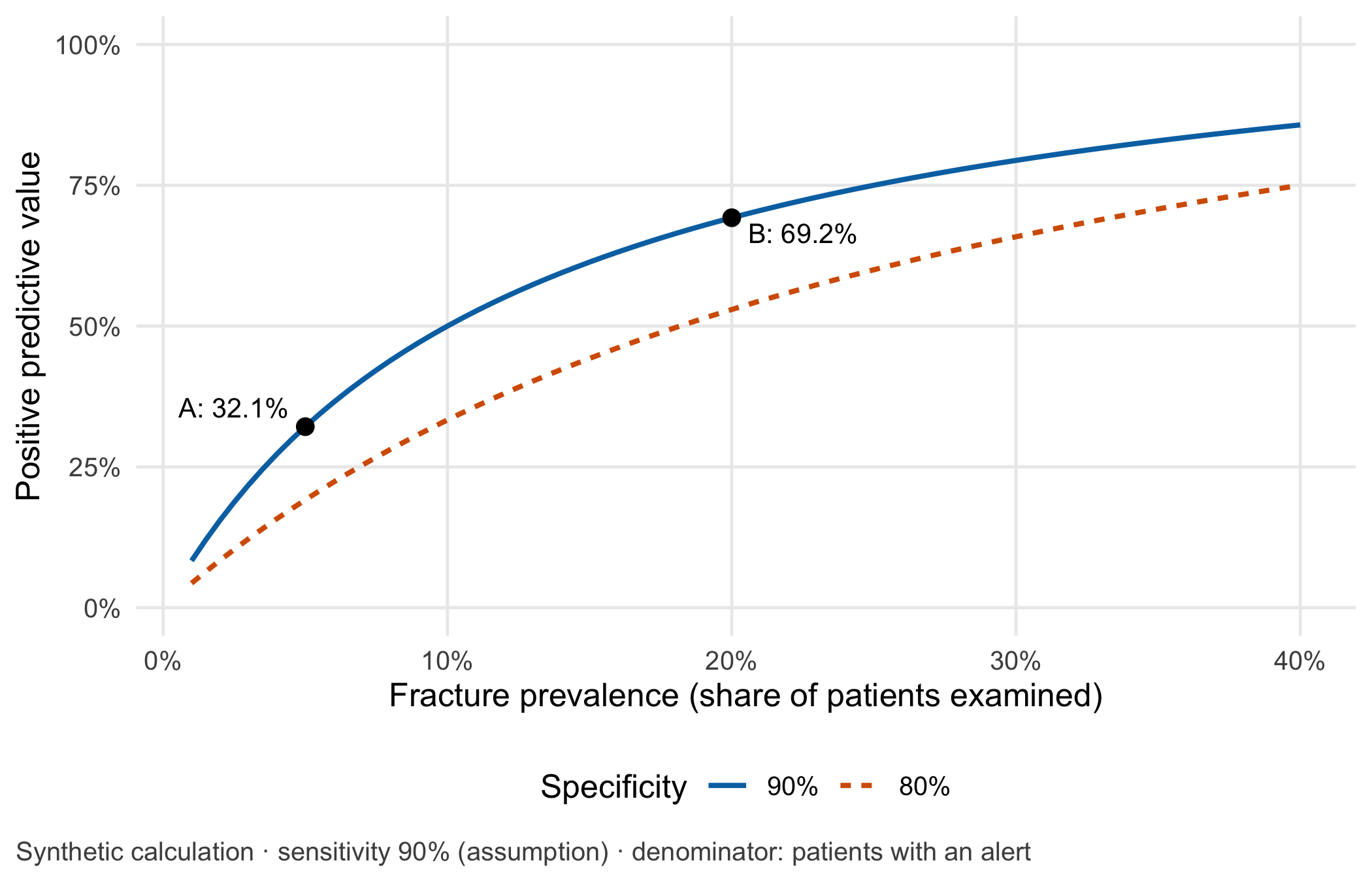
A second counter-check changes the target population instead of the tool. If the tool were used for all radiographs in a children’s emergency department, which numbers in the table would you have to measure again before reusing any of them? (All four cells: prevalence, injury pattern, image appearance and the reference standard can all differ.)
9.5 Consequences for patients and operations
Ethics. False alerts are not free. Patients may wait longer, receive an extra view or a CT scan with additional radiation, or leave with a splint they did not need. Clinicians who see many uninformative alerts start to ignore them: in one primary care study, acceptance of reminders fell with each additional reminder per encounter and with the share of repeated reminders [Ancker et al. (2017); published]. The opposite risk is automation bias: a missing box may be read as an all-clear. Who carries which share of these harms, and how uncertainty is explained to a patient, is the subject of Chapter 21.
Regulation. The intended purpose decides the regulatory question, not the calculation. Software “intended to provide information which is used to take decisions with diagnosis or therapeutic purposes” is classified at least as class IIa under Rule 11 of Annex VIII of the Medical Device Regulation (EU) 2017/745 [European Parliament and Council of the European Union (2017); binding text]. An AI system that is itself a medical device and has to undergo third-party conformity assessment is a high-risk AI system under Article 6(1) of the AI Act, Regulation (EU) 2024/1689 [European Parliament and Council of the European Union (2024); binding text]. Since the amending Regulation (EU) 2026/1744 (published 24 July 2026, in force since 27 July 2026), the obligations of Chapter III, Sections 1 to 3, apply to such systems from 2 August 2028 [European Parliament and Council of the European Union (2026); binding text]. Whether the fictitious tool in this chapter is such a device, and who would be manufacturer and who deployer, is examined in Chapter 22 by reading its intended purpose. Status: November 2026.
Data protection. The local pilot needs images, tool outputs and reference diagnoses. Whether an external service provider needs the original images for this evaluation, or whether derived and minimised data suffice, is decided in Chapter 23.
Information security and operations. If the tool fails or an unapproved model version is installed, reporting must continue by the regular route without delay. Chapter 24 designs a failure test and that fallback; Chapter 20 uses alerts per shift as a monitoring signal.
The case returns four times. In Chapter 21 a patient, a nurse and a researcher judge the same alert and the distribution of false alerts. In Chapter 22 teams read the fictitious intended purpose. In Chapter 23 they decide whether a service provider needs the original images. In Chapter 24 they design a failure test and a safe route back to regular reporting.
9.6 Look up and transfer
- Reviewer question: The manuscript reports a PPV of 70%. In which population was it measured, what was the prevalence, and was that prevalence fixed by the study design?
- Self-test: A smaller emergency department wants to use the tool only at night. It performs 400 limb radiographs per month on 30 night shifts. Assume a fracture prevalence of 10%, a sensitivity of 90% and, because of older equipment, a specificity of 80%. How many alerts and how many false alerts arise per night, what is the PPV, and should the department switch the tool off because the PPV is “only one third”?
TipAnswer
Of 400 patients, 40 have a fracture: 36 are flagged and 4 are missed. Of the 360 without a fracture, 72 are flagged and 288 are not. There are 108 alerts, so the PPV is 36/108 = 33.3% and the NPV 288/292 = 98.6%. Per night shift this means 3.6 alerts, 2.4 of them false. The PPV alone does not justify switching the tool off. The department needs to know how long a second look takes at night, how many of the 36 flagged fractures the night team would otherwise have missed, and whether the specificity of 80% reflects a local equipment problem that could be fixed. With fourfold(0.10, 0.90, 0.80, examined = 400) the lab function reproduces these numbers.
- Annotated sources:
- Leeflang et al. (2013) supports the warning that sensitivity and specificity need not be transferable between settings with different prevalence.
- Hoffrage et al. (2000) is the reason why the chapter counts people before it computes percentages.
- Altman and Bland (1994) is the classic short explanation of predictive values and their dependence on prevalence.
- Guermazi et al. (2022) is the published example of a reader study with prevalence fixed by design.
- Vickers and Elkin (2006) introduces net benefit, the decision-analytic view behind “a lower PPV is not a verdict”.
- Ancker et al. (2017) provides published evidence that more and repeated alerts are accepted less often.
- Sounderajah et al. (2025) and Vasey et al. (2022) are the reporting guidelines for accuracy studies and early clinical evaluation.
- European Parliament and Council of the European Union (2017), European Parliament and Council of the European Union (2024) and European Parliament and Council of the European Union (2026) are the binding legal texts behind the regulatory paragraph.
9.7 Further reading
- Chapter 6 – thresholds, calibration and net benefit for the same fourfold logic.
- Chapter 7 – how to read a diagnostic AI study with STARD-AI before trusting its PPV.
- Chapter 20 – alerts per shift as a monitoring signal during a pilot.
- Chapter 21 – the same alert from the perspectives of patient, nurse and researcher.
- Methods in R: Diagnostic Test Accuracy – sensitivity, specificity and their confidence intervals.
- Methods in R: Power for Diagnostic Accuracy – how many patients a local accuracy study would need.
- CTTIR Courses: Diagnostic testing: Se, Sp, PPV, NPV, LR – a lab with likelihood ratios as the next step.
- CTTIR Tutorials: Diagnostic Test Accuracy – a compact tutorial for revision.