R. Heller · Date: 2025-05-18 · Last changed: 2026-11-09
NoteAt a glance
Guiding question: Are two measurement methods similar enough for this rehabilitation decision? For: physiotherapists, rehabilitation and trauma clinicians, and researchers who compare a new measurement method with an established one. · Prerequisites: repeated measurements and the unit of analysis from Chapter 3; the measurement chain from Chapter 10. In the course:W4 · What imaging, gait and tissue models measure (gait station) and W5 · Causal questions, trajectories and phenotypes · Data: synthetic (generated in the chapter) · Core reading time: about 10 minutes
11.1 Case and decision
A physiotherapist in a fictitious rehabilitation clinic follows patients after surgery for a tibial plateau fracture. One criterion for moving a patient to the next stage of the gait programme is the peak knee flexion during the swing phase. Until now it has been measured in the gait laboratory with a marker-based motion capture system, which is booked out for weeks. A smartphone video analysed by a pose-estimation model would take five minutes on the ward. In the first trial recordings the video values are systematically lower for some patients. Looking at the setup, the physiotherapist notices that the phone stood at an angle to the walkway because the corridor is narrow. She has to decide whether the video method may replace the laboratory measurement for this decision, and under which conditions. The first error in this chapter is the perspective.
11.2 Core reading
Core reading · recommended reading for W4 (gait station) · about 10 minutes · ends before ‘Lab’
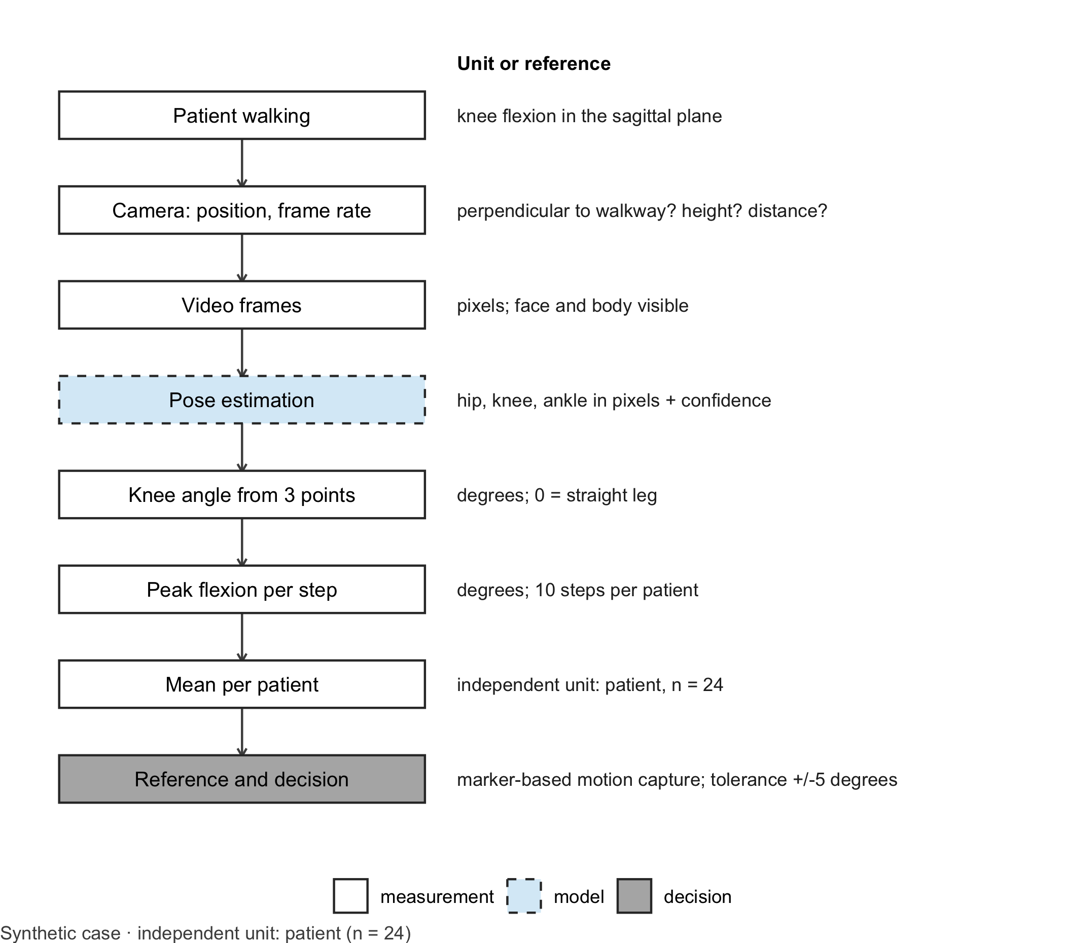
From pixels to degrees. A pose-estimation model is a learning model that finds anatomical landmarks in each video frame, for example hip, knee and ankle, and returns their pixel coordinates with a confidence score (Mathis et al. 2018). Everything after that is geometry. The knee angle at one moment is the angle between the thigh (knee to hip) and the shank (knee to ankle). Knee flexion is 180° minus that angle: 0° for a straight leg. Over a gait cycle the flexion rises to a peak in the swing phase; that peak, in degrees, is the quantity the clinic wants. Figure 11.1 shows the whole chain and where the learning model sits.
Code
library(ggplot2)# Generic drawing of a measurement chain: one box per step, a note per step, dashed border for the learning modeldraw_chain <-function(steps, note_title ="Unit or reference") { steps$y <-rev(seq_len(nrow(steps))) types <-c("measurement", "reference", "model", "decision")ggplot(steps) +geom_segment(data = steps[-nrow(steps), ], aes(x =1, xend =1, y = y -0.24, yend = y -0.76),arrow = grid::arrow(length = grid::unit(0.15, "cm")), colour ="grey30") +geom_tile(aes(x =1, y = y, fill = type, linetype = type), width =1.7, height =0.5,colour ="grey20", linewidth =0.5) +geom_text(aes(x =1, y = y, label = label), size =3.4) +geom_text(aes(x =2.0, y = y, label = note), hjust =0, size =3.1, colour ="grey15") +annotate("text", x =2.0, y =nrow(steps) +0.55, label = note_title, hjust =0, fontface ="bold",size =3.2) +scale_fill_manual(values =c(measurement ="white", reference ="grey85", model ="#D9ECF7",decision ="grey70"), breaks = types, name =NULL) +scale_linetype_manual(values =c(measurement ="solid", reference ="solid", model ="dashed",decision ="solid"), breaks = types, name =NULL) +scale_x_continuous(limits =c(0.1, 4.6)) +scale_y_continuous(limits =c(0.5, nrow(steps) +0.8)) +theme_void(base_size =11) +theme(legend.position ="bottom", plot.caption =element_text(hjust =0, colour ="#4D4D4D"))}chain_b11 <-data.frame(label =c("Patient walking", "Camera: position, frame rate", "Video frames", "Pose estimation","Knee angle from 3 points", "Peak flexion per step", "Mean per patient", "Reference and decision"),note =c("knee flexion in the sagittal plane", "perpendicular to walkway? height? distance?","pixels; face and body visible", "hip, knee, ankle in pixels + confidence","degrees; 0 = straight leg", "degrees; 10 steps per patient", "independent unit: patient, n = 24","marker-based motion capture; tolerance +/-5 degrees"),type =c("measurement", "measurement", "measurement", "model", "measurement", "measurement", "measurement","decision"))draw_chain(chain_b11) +labs(caption ="Synthetic case · independent unit: patient (n = 24)")
Figure 11.1: Measurement chain for knee flexion from video. The dashed box marks the learning model (pose estimation); the dark grey box marks the comparison with the reference method and the decision. Unit: degrees from step 5 onwards. Independent unit for the agreement question: patient (n = 24 in the lab, ten steps each). Synthetic case.
Code: geometry for the perspective figure
# Geometry used in the core reading (the lab explains the same functions step by step)knee_flexion <-function(hip, knee, ankle) { hip <-matrix(hip, ncol =2); knee <-matrix(knee, ncol =2); ankle <-matrix(ankle, ncol =2) v1 <- hip - knee; v2 <- ankle - knee cos_angle <-rowSums(v1 * v2) /sqrt(rowSums(v1^2) *rowSums(v2^2))180-acos(pmin(pmax(cos_angle, -1), 1)) *180/ pi}landmarks <-function(hip_flex, knee_flex, thigh =0.43, shank =0.42) { r <- pi /180 knee <-cbind(thigh *sin(hip_flex * r), -thigh *cos(hip_flex * r)) ankle <- knee +cbind(shank *sin((hip_flex - knee_flex) * r), -shank *cos((hip_flex - knee_flex) * r))list(hip =cbind(0* hip_flex, 0* hip_flex), knee = knee, ankle = ankle)}project <-function(p, yaw) cbind(p[, 1] *cos(yaw * pi /180), p[, 2])seen <-function(knee_flex, yaw, hip_flex =20) { L <-landmarks(hip_flex, knee_flex)knee_flexion(project(L$hip, yaw), project(L$knee, yaw), project(L$ankle, yaw))}proj_30_60 <-seen(60, 30)
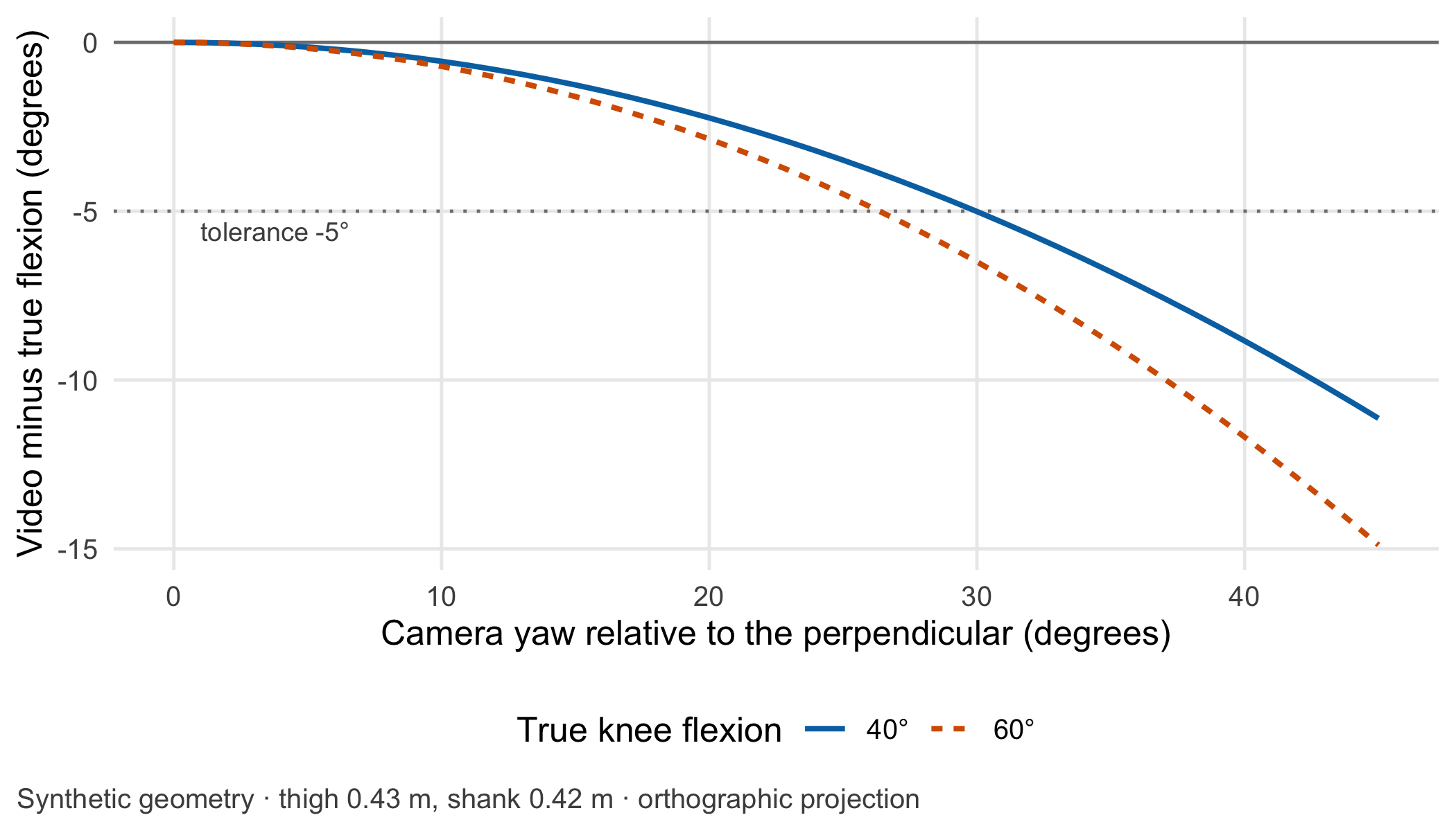
The perspective error. A single camera sees a flat projection of a three-dimensional movement. If it looks at the walkway at a right angle, the sagittal plane is projected without distortion. If the phone is turned by a yaw angle, all forward-backward distances in the image shrink by the cosine of that angle while vertical distances stay. Thigh and shank then look more vertical than they are, and the knee looks straighter. Figure 11.2 computes this for a simplified setup without lens distortion: at a yaw of 30°, a true flexion of 60° appears as about 53.5°. The error is systematic, not random. Repeating the recording does not average it away, and it is larger in patients who bend the knee more.
Figure 11.2: Systematic error of video-based knee flexion when the camera is turned away from the perpendicular, for true flexion of 40° and 60° (hip flexion 20°; simplified orthographic projection). Unit: degrees. Synthetic geometry, no patients involved.
What the pose model knows. The pose-estimation model was trained on labelled images, most of them of people in everyday scenes. It has not necessarily seen crutches, knee braces, compression stockings or a far leg hidden behind the near one (occlusion). Each of these can shift the knee landmark by a centimetre or two, and with a thigh of about 43 cm that already moves the angle by a few degrees. A low confidence score is a warning, not a correction. The model is the only learned step in the chain; everything after it is geometry that can be checked by hand, as the lab does with two angles worked out on paper.
Reference and unit. The comparison method is the laboratory’s marker-based motion capture. It is itself a measurement with its own error, not the truth, so an agreement study compares two methods and assumes neither to be perfect. The physical unit is the degree throughout. The independent unit is the patient: 24 patients with ten steps each in the lab.
Agreement, not correlation. To decide whether the video can replace the laboratory, the clinic records the same steps with both methods and looks at the differences. The Bland–Altman approach plots the difference of the two methods against their mean, estimates the average difference (bias) and the limits of agreement, within which about 95% of differences are expected (Bland and Altman 1986). A high correlation would say nothing useful: two methods can correlate perfectly while one reads 10° lower. Details are in Methods in R: Bland-Altman Limits of Agreement.
Set the tolerance before looking. Whether the limits of agreement are good enough is a clinical judgement, not a statistical one, and it has to be made before the data are seen. In the fictitious protocol the progression criteria are set in steps of 10°, so the team decides that a patient’s value may differ from the laboratory value by at most half a step. The key assumption is a tolerance of ±5° for the value on which the decision is based (assumption, to be agreed locally). Published comparisons of two-dimensional video with motion capture report mean absolute errors of several degrees for sagittal knee angles, so the question is realistic [Stenum et al. (2021); published].
Which value is the decision based on? Each patient contributes ten steps. Steps of the same patient are not independent: they share the person, the camera setup and the clothing. The independent unit is the patient. Two analyses are legitimate, and they answer different questions. If the decision uses a single step, the limits of agreement must describe single steps; with repeated steps per patient they are estimated from the within-patient and between-patient variance components (Bland and Altman 2007). If the decision uses the mean of ten steps, the limits must describe ten-step means, one per patient. Pooling all 240 steps as if they came from 240 patients is not legitimate: it makes the uncertainty of the bias look smaller than it is. Which level applies, and how many steps a recording must contain, is written into the protocol before the comparison starts.
Question for the workshop: Your clinic uses the mean of ten steps. Which of the two sets of limits of agreement belongs in the clinical protocol, and what would have to change in the protocol if the ward only recorded three steps?
11.3 Lab
The lab simulates 24 fictitious patients with ten steps each, measured simultaneously by a marker-based reference and by a video method whose landmarks carry noise and a small systematic offset. It then checks agreement at both decision levels.
Step 1 – the angle from three points. The function accepts single points or one row per step and is checked against two angles that can be worked out by hand.
# Knee flexion in degrees from 2D hip, knee and ankle coordinates (x forward, z up); 0 = straight legknee_flexion <-function(hip, knee, ankle) { hip <-matrix(hip, ncol =2); knee <-matrix(knee, ncol =2); ankle <-matrix(ankle, ncol =2) thigh_vec <- hip - knee # from knee to hip shank_vec <- ankle - knee # from knee to ankle cos_angle <-rowSums(thigh_vec * shank_vec) /sqrt(rowSums(thigh_vec^2) *rowSums(shank_vec^2))180-acos(pmin(pmax(cos_angle, -1), 1)) *180/ pi # flexion = 180 degrees minus the inner angle}stopifnot(abs(knee_flexion(c(0, 0), c(0, -1), c(0, -2)) -0) <1e-9, # straight leg: 0 degreesabs(knee_flexion(c(0, 0), c(0, -1), c(-1, -1)) -90) <1e-9# shank horizontal: 90 degrees)knee_flexion(c(0, 0), c(0.15, -0.40), c(-0.20, -0.65)) # an arbitrary example in metres
#> [1] 75.01837
Step 2 – synthetic patients and steps. Landmarks are generated in the sagittal plane, projected for the camera’s yaw, offset and blurred like a pose-estimation output, and then turned back into angles.
set.seed(1111)n_patients <-24n_steps <-10patients <-data.frame(patient =sprintf("P%02d", 1:n_patients),mean_flexion =rnorm(n_patients, 55, 7), # true peak swing flexion per patient (degrees)hip_flexion =rnorm(n_patients, 20, 3), # hip flexion at that moment (degrees)yaw =runif(n_patients, -5, 5), # camera almost perpendicular (degrees)knee_offset =rnorm(n_patients, 0.004, 0.006), # knee landmark placed slightly anterior (metres)size =rnorm(n_patients, 1, 0.05) # body size factor for segment lengths)# Landmarks in metres for given hip and knee flexion; projection for a camera turned by 'yaw' degreeslandmarks <-function(hip_flex, knee_flex, thigh =0.43, shank =0.42) { r <- pi /180 knee <-cbind(thigh *sin(hip_flex * r), -thigh *cos(hip_flex * r)) ankle <- knee +cbind(shank *sin((hip_flex - knee_flex) * r), -shank *cos((hip_flex - knee_flex) * r))list(hip =cbind(0* hip_flex, 0* hip_flex), knee = knee, ankle = ankle)}project <-function(p, yaw) cbind(p[, 1] *cos(yaw * pi /180), p[, 2])simulate_steps <-function(patients, yaw) { rows <-lapply(seq_len(nrow(patients)), function(i) { true <- patients$mean_flexion[i] +rnorm(n_steps, 0, 2.5) # step-to-step variation hip <- patients$hip_flexion[i] +rnorm(n_steps, 0, 2) L <-landmarks(hip, true, 0.43* patients$size[i], 0.42* patients$size[i]) L$knee[, 1] <- L$knee[, 1] + patients$knee_offset[i] # systematic landmark offset blur <-function() matrix(rnorm(2* n_steps, 0, 0.012), ncol =2) # landmark noise, metres video <-knee_flexion(project(L$hip, yaw[i]) +blur(), project(L$knee, yaw[i]) +blur(),project(L$ankle, yaw[i]) +blur())data.frame(patient = patients$patient[i], step =1:n_steps, true = true,reference = true +rnorm(n_steps, 0, 1), # marker-based referencevideo = video) }) steps <-do.call(rbind, rows) steps$difference <- steps$video - steps$reference steps}steps <-simulate_steps(patients, patients$yaw)gait_file <- steps[, c("patient", "step", "reference", "video")]gait_file[, c("reference", "video")] <-round(gait_file[, c("reference", "video")], 2) # degrees, 2 decimalswrite.csv(gait_file, "../data/b11-gait-steps.csv", row.names =FALSE)c(patients =length(unique(steps$patient)), steps =nrow(steps))
#> patients    steps
#>       24      240
The file data/b11-gait-steps.csv holds the synthetic reference and video values for the gait station in W4; the true values stay in the simulation.
Step 3 – agreement at both decision levels. The single-step limits use the variance components of Bland and Altman’s method for repeated measurements in which the true value varies (Bland and Altman 2007). The ten-step limits use one mean difference per patient.
tolerance <-5# degrees, set before the analysis (assumption)# (a) Single steps: one-way ANOVA of the differences by patientfit <-anova(lm(difference ~ patient, data = steps))ms_within <- fit["Residuals", "Mean Sq"]ms_between <- fit["patient", "Mean Sq"]var_between <-max(0, (ms_between - ms_within) / n_steps)bias <-mean(steps$difference)sd_single <-sqrt(var_between + ms_within)# (b) Ten-step means: one value per patientper_patient <-aggregate(cbind(reference, video, difference) ~ patient, data = steps, FUN = mean)sd_mean10 <-sd(per_patient$difference)# Confidence interval of the bias: patients are the independent unit (n = 24), not steps (n = 240)ci_patients <- bias +c(-1, 1) *qt(0.975, n_patients -1) * sd_mean10 /sqrt(n_patients)ci_steps_wrong <- bias +c(-1, 1) *qt(0.975, nrow(steps) -1) *sd(steps$difference) /sqrt(nrow(steps))agreement <-data.frame(decision_level =c("single step", "mean of 10 steps"),bias = bias, lower_loa = bias -1.96*c(sd_single, sd_mean10), upper_loa = bias +1.96*c(sd_single, sd_mean10))agreement$within_tolerance <- agreement$lower_loa >=-tolerance & agreement$upper_loa <= toleranceagreement
#>     decision_level     bias lower_loa upper_loa within_tolerance
#> 1      single step 1.290632 -6.030212  8.611475            FALSE
#> 2 mean of 10 steps 1.290632 -1.395141  3.976405             TRUE
stopifnot(agreement$within_tolerance ==c(FALSE, TRUE),diff(ci_patients) >diff(ci_steps_wrong)) # pooling steps understates the uncertainty
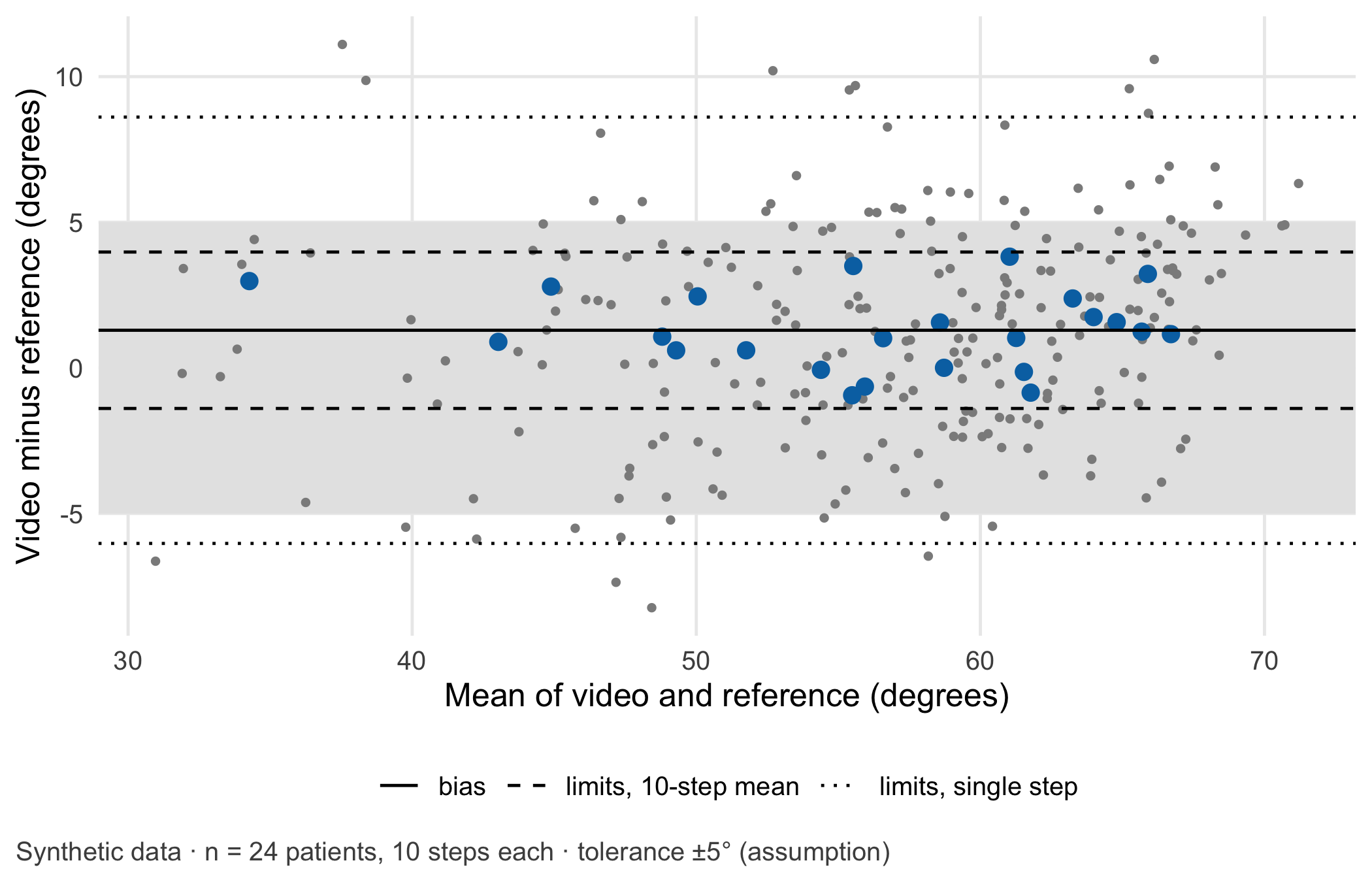
For single steps the limits of agreement run from -6° to 8.6° and exceed the tolerance. For the ten-step mean they run from -1.4° to 4° and lie within it. The video method, recorded perpendicular to the walkway, is acceptable for a decision based on ten steps and not for one based on a single step. The confidence interval for the bias based on 24 patients (0.7° to 1.9°) is wider than the one obtained by pretending that 240 steps were 240 patients (0.8° to 1.8°).
WarningCommon mistake
Averaging the ten steps per patient first and then quoting the resulting limits of agreement as if they applied to single measurements. Limits of agreement belong to the quantity on which they were computed: limits for ten-step means are narrower than limits for single steps and must not be used for a protocol that relies on one step.
Code
steps$mean_methods <- (steps$video + steps$reference) /2per_patient$mean_methods <- (per_patient$video + per_patient$reference) /2lines_ba <-data.frame(y =c(bias, agreement$lower_loa[2], agreement$upper_loa[2], agreement$lower_loa[1], agreement$upper_loa[1]),type =c("bias", "limits, 10-step mean", "limits, 10-step mean", "limits, single step","limits, single step"))ggplot() +annotate("rect", xmin =-Inf, xmax =Inf, ymin =-tolerance, ymax = tolerance, fill ="grey90") +geom_point(data = steps, aes(mean_methods, difference), colour ="grey55", size =0.9) +geom_point(data = per_patient, aes(mean_methods, difference), colour = cdsr_colours["blue"], size =2.8,shape = cdsr_shapes[1]) +geom_hline(data = lines_ba, aes(yintercept = y, linetype = type)) +scale_linetype_manual(values =c("bias"="solid", "limits, 10-step mean"="dashed","limits, single step"="dotted"), name =NULL) +labs(x ="Mean of video and reference (degrees)", y ="Video minus reference (degrees)",caption ="Synthetic data · n = 24 patients, 10 steps each · tolerance ±5° (assumption)") +theme_cdsr()
Figure 11.3: Bland–Altman plot for peak knee flexion, video minus marker-based reference, in degrees. Large symbols: ten-step means per patient (n = 24 independent patients); small grey dots: single steps (240). Solid line: bias; dashed lines: limits of agreement for ten-step means; dotted lines: limits for single steps; shaded band: pre-specified tolerance of ±5° (assumption). Synthetic data.
NoteOther implementation: Python with PyTorch
Pose estimation itself is rarely written in R. The PyTorch library torchvision offers a Keypoint R-CNN model with weights trained on the COCO person keypoints (KeypointRCNN_ResNet50_FPN_Weights.COCO_V1), which returns 17 keypoints per person, including both hips, knees and ankles, as [x, y, visibility] in pixel coordinates; inputs are expected as tensors scaled to the range 0–1 (Paszke et al. 2019). For landmarks that COCO does not define, such as markers on a brace, DeepLabCut trains a network on a few hundred hand-labelled frames (Mathis et al. 2018). The concrete advantage is a tested detector with known weights instead of hand-placed points. To compare it fairly with this lab, the following must be identical and recorded: the video frames (frame rate, resolution and the phone’s rotation metadata), the mapping from keypoint index to hip, knee and ankle of the correct side, the handling of low-confidence keypoints, the definition of a step and its peak, the averaging over ten steps, the metric (difference to the reference in degrees) and the tolerance of ±5°. Weights and software version (torchvision 0.29.2 or DeepLabCut 3.0.2 in November 2026) belong in the model passport. Status: conceptual comparison, not run.
11.4 Counter-check
Now reproduce the error from the case. For the first eight patients the phone stands at 30° to the walkway; the remaining sixteen are recorded as before. Predict first: does the bias move up or down, and do the ten-step limits of agreement stay within ±5°?
The bias in the turned setup is -4.9° against 1.1° with a perpendicular camera, and the lower limit of agreement of the ten-step means falls to -7.2°, outside the tolerance. The perspective error is systematic, so averaging steps does not remove it. The plausible failure mode is therefore concrete: a phone placed at an angle underestimates knee flexion, most in patients with the largest flexion, and may hold patients back in the programme. The checkable measurement assumption is equally concrete: the camera axis is perpendicular to the walkway within ±10°, verified with a floor marking and a photo of the setup for every recording.
11.5 Consequences for patients and operations
An identifiable movement pattern. A gait video shows face, body and clothing, and it is health data. Removing the face is not enough: gait patterns are so individual that learning models can attribute them to single persons from joint angles and forces alone [Horst et al. (2019); published]. The derived keypoint trajectories may therefore still identify a patient, especially combined with ward and date. The General Data Protection Regulation (EU) 2016/679 (GDPR) defines biometric data as personal data resulting from specific technical processing of physical, physiological or behavioural characteristics “which allow or confirm the unique identification” of a person (Article 4(14)); Article 9(1) lists biometric data “for the purpose of uniquely identifying a natural person” and data concerning health among the special categories [European Parliament and Council of the European Union (2016); binding text]. Whether the keypoint data in this case fall under the biometric category is a question of interpretation for the data protection officer; that in this clinical context they are data concerning health (Article 4(15)) is hardly in doubt. The decision the team has to take is practical: does the clinic need the raw video for its purpose, for example to audit implausible angles, and if so, for how long? Chapter 23 follows exactly this data flow from video to angle and deletion point.
Regulation. If the clinic used the app’s output to decide a patient’s progression, the intended purpose stated by the manufacturer would determine whether the software is a medical device and of which class (Rule 11 of Annex VIII of the MDR (European Parliament and Council of the European Union 2017)). An app marketed for “fitness tracking” and used for a clinical decision raises its own question. Chapter 22 works through such intended purposes.
Ethics and operations. A systematic underestimation does not hit everyone alike: it is largest in patients with the largest flexion and in wards with the narrowest corridors. The patient sees only “not yet”. A short note in the protocol on camera setup, and a re-measurement in the laboratory when the video value lies within 5° of a decision threshold, keep the faster method without shifting its errors onto patients.
11.6 Look up and transfer
Reviewer question: The study reports limits of agreement of ±4° from 600 steps of 30 participants. Were the limits computed for single steps or for participant means, how were repeated steps handled, and was the tolerance defined before the analysis?
Self-test: The ward wants to record only three steps per patient. Using the variance components from the lab, estimate the limits of agreement for a three-step mean. Is the video method still acceptable at a tolerance of ±5°?
TipAnswer
For the mean of \(m\) steps the variance of a patient’s mean difference is the between-patient component plus the within-patient component divided by \(m\). With the lab’s values (between-patient variance 0.54, within-patient variance 13.41, both in squared degrees) a three-step mean has a standard deviation of 2.24° and limits of agreement from -3.1° to 5.7°. In R: bias + c(-1.96, 1.96) * sqrt(var_between + ms_within / 3). The upper limit exceeds +5°, so at this tolerance the video method is not acceptable for a three-step protocol, although it is for ten steps. A protocol based on three steps needs its own agreement statement and must not reuse the ten-step limits. The estimate also assumes that three steps on the ward vary like ten steps in the laboratory, which itself is an assumption to check.
Annotated sources:
Bland and Altman (1986) introduced limits of agreement and explains why correlation is the wrong tool.
Bland and Altman (2007) provides the variance-components method for several observations per person used in the lab.
Stenum et al. (2021) compares two-dimensional video pose estimation with motion capture on a stride-by-stride basis and shows realistic error sizes for sagittal knee angles.
Mathis et al. (2018) describes markerless pose estimation of user-defined landmarks with a learning model.
Horst et al. (2019) supports the statement that individual gait patterns are distinctive enough to identify people.
European Parliament and Council of the European Union (2016) is the binding text for the definitions of biometric and health data.
11.7 Further reading
Chapter 23 – the data flow from gait video to angle, service provider and deletion point.
Chapter 13 – repeated measurements over time and the person as the unit of analysis.
Chapter 10 – the measurement chain of a second imaging method, where the first error is the light.
Bland, J. Martin, and Douglas G. Altman. 1986. “Statistical Methods for Assessing Agreement Between Two Methods of Clinical Measurement.”The Lancet 327 (8476): 307–10. https://doi.org/10.1016/S0140-6736(86)90837-8.
Bland, J. Martin, and Douglas G. Altman. 2007. “Agreement Between Methods of Measurement with Multiple Observations Per Individual.”Journal of Biopharmaceutical Statistics 17 (4): 571–82. https://doi.org/10.1080/10543400701329422.
Horst, Fabian, Sebastian Lapuschkin, Wojciech Samek, Klaus-Robert Müller, and Wolfgang I. Schöllhorn. 2019. “Explaining the Unique Nature of Individual Gait Patterns with Deep Learning.”Scientific Reports 9 (1): 2391. https://doi.org/10.1038/s41598-019-38748-8.
Mathis, Alexander, Pranav Mamidanna, Kevin M. Cury, Taiga Abe, et al. 2018. “DeepLabCut: Markerless Pose Estimation of User-Defined Body Parts with Deep Learning.”Nature Neuroscience 21 (9): 1281–89. https://doi.org/10.1038/s41593-018-0209-y.
Stenum, Jan, Cristina Rossi, and Ryan T. Roemmich. 2021. “Two-Dimensional Video-Based Analysis of Human Gait Using Pose Estimation.”PLOS Computational Biology 17 (4): e1008935. https://doi.org/10.1371/journal.pcbi.1008935.