19 From one centre or species to the next
R. Heller · Date: 2025-09-28 · Last changed: 2026-11-09
19.1 Case and decision
A doctoral researcher in a preclinical imaging group presents a slide at the lab meeting: a classifier separates two tissue classes, A and B, in hyperspectral reflectance spectra, and the test accuracy is 100%. The data come from four animals with three spectra each. The group leader wants to quote the result in a funding application for a first feasibility study in patients with soft-tissue injuries. Before the sentence goes into the application, a methods reviewer in the group asks one question: which new case was the test about? A further spectrum from an animal that the model has already seen, a new animal from the same laboratory, an animal measured next year with a new camera, or a patient? The answer decides what the group may write. If the test only measured recognition of known animals, the application would ask patients to carry the burden of a study whose central premise was never tested.
19.2 Core reading
Every test answers a question about a particular kind of new case. A model evaluated on new spectra from animals it has already seen answers the question “does it recognise more data from these animals?”. A model evaluated on animals it has never seen answers “does it work for a new animal from the same setting?”. Neither answers “does it work in another centre, with another device, or in another species?”. The skill this chapter trains is to name the intended new case before choosing the split, and then to check that the split really produces such cases.
Five levels of “new”. It helps to list the levels explicitly (Table 19.1). Each row needs its own test, and a positive result on an upper row says nothing about the rows below it. The general idea of keeping training and test data apart is covered in Chapter 5 and in Methods in R: Train-Test Splits; here the point is which unit must be new.
| Intended new case | Split that produces it | Independent denominator |
|---|---|---|
| Another spectrum or image of a known animal | Image-wise: spectra of each animal on both sides | Spectra (but they are not independent) |
| A new animal, same laboratory and device | Animal-wise (group split): every animal on one side only | Animals in the test set |
| A later animal, after protocol drift | Temporal: train on earlier, test on later animals | Animals measured after the cut-off |
| Another centre, device or operator | External: develop at one site, test at another | Animals (or patients) at the new site |
| Another species, or patients | A new study in the target population | Individuals of the target species |
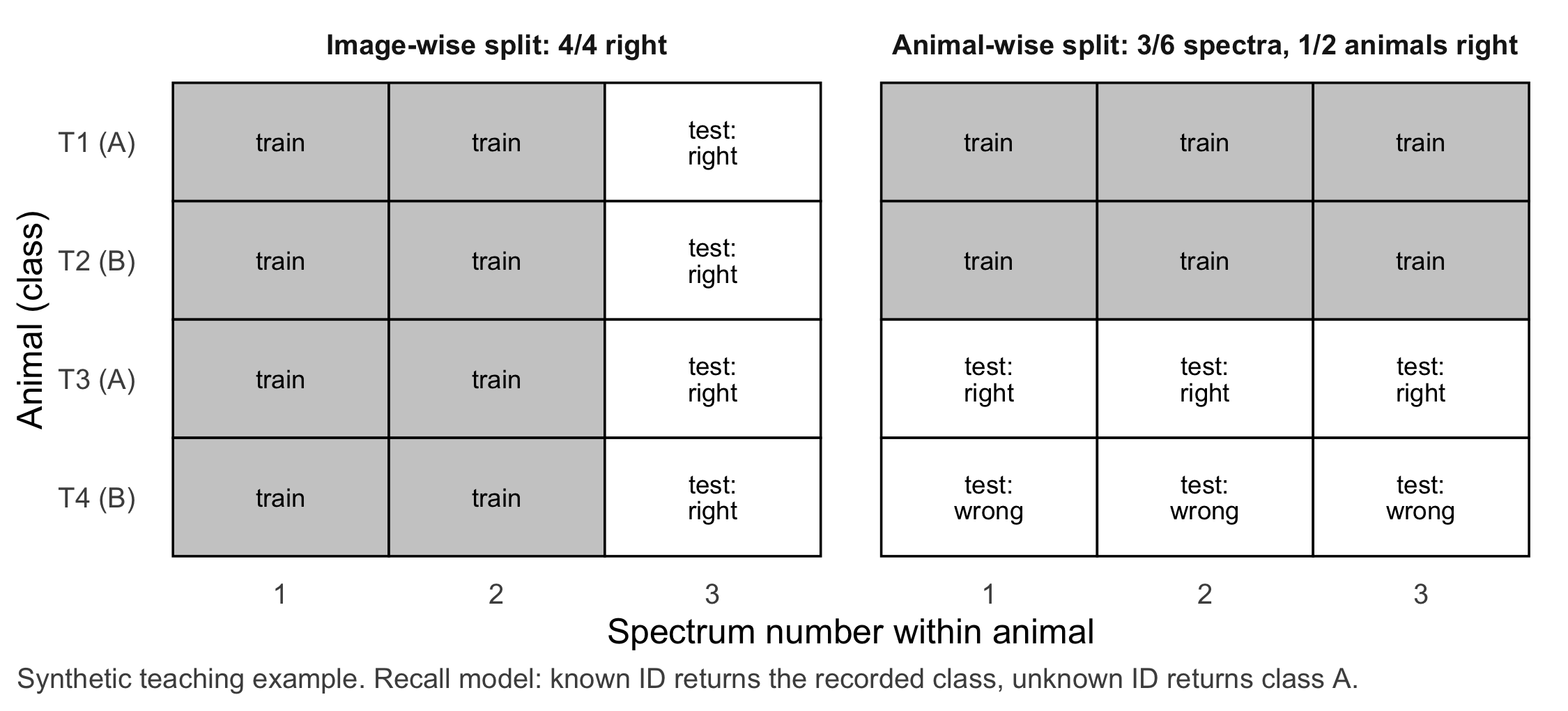
A deliberately trivial example. Four fictitious animals, T1 to T4, each contribute three spectra. The classes are properties of animals: T1 and T3 belong to class A, T2 and T4 to class B. Instead of a real classifier we use a didactic model that is constructed to cheat in a transparent way. It never looks at a spectrum. For an animal ID it has seen during training, it returns the class it recorded for that animal. For any other ID it returns a fallback class that was fixed in advance: class A. Call it the recall model. If a test cannot distinguish this model from a useful one, the test is not informative about new animals.
What the two designs show. In the image-wise split, two spectra of every animal are used for training and the third for testing. Every test ID is known, so the recall model gets 4 of 4 right. It has measured recognition, not classification. In the animal-wise split, T1 (A) and T2 (B) are used for training; T3 (A) and T4 (B) with three spectra each form the test set. Both IDs are unknown, so the fallback class A is returned six times: 3 of 6 spectra are right, and at the level of animals 1 of 2. The independent denominator is two animals, not six spectra. A result of “50%” from two animals is compatible with almost anything; it is a statement about two individuals.
The most important assumption. A test is informative about the intended new case only if the unit that is new in the test is the unit that the claim is about, and the denominator counts those units. For a claim about new animals the test must contain animals the model has never seen, and accuracy must be reported per animal. In R this is one line: intersect(unique(train$id), unique(test$id)) must be empty for the animal-wise split. The same leak appears under many names in the literature, from pseudoreplication to “data leakage” (Kapoor and Narayanan 2023), and grouped or blocked cross-validation is the standard remedy for clustered data (Roberts et al. 2017).
Beyond the group split. An empty ID intersection is necessary, not sufficient. A clinical prediction model can be reproducible in new patients from the same population yet fail to be transportable to a different but related population (Justice et al. 1999). External validation is therefore interpreted against the difference in case mix between development and validation samples (Debray et al. 2015). Two further shifts matter in imaging. A change in measurement procedure (camera, illumination, calibration, operator) can alter spectra in ways that a model learns as if it were biology; an imaging model for chest radiographs, for example, could identify the hospital system of a radiograph almost perfectly, which can confound its predictions (Zech et al. 2018). And a change of species is not a larger version of a change of centre. Whether mouse models “mimic” human inflammatory responses after trauma and burns has been answered in opposite directions from the same gene expression data, depending on which genes were compared (Seok et al. 2013; Takao and Miyakawa 2015). The lesson for this chapter is modest: similarity between species is a claim with its own analysis choices, and a model trained in animals makes no claim about patients until it has been tested in patients.
What the reviewer writes back. “The 100% result is an image-wise test. It supports the statement that spectra of the four known animals can be recognised. For new animals, the independent denominator is the number of test animals; please report the animal-wise result with its denominator. A statement about patients needs a study in patients.” The finding is not worthless. It is an honest description of what was tested, and it points to the next study, which in preclinical work also has to justify the number of animals under the 3Rs (Chapter 16).
Question for the workshop: Your group has spectra from six animals measured in two laboratories with two cameras. Write down the intended new case for your claim, the split that produces it, and the denominator you would report. Which row of Table 19.1 can your data not reach at all?
19.3 Lab
The lab has three parts. First, the hand calculation from the core reading is reproduced exactly, with target values. Second, a self-contained variant uses a nearest-neighbour model on synthetic spectra with the same animal IDs; its results are kept in separate objects. Third, a deepening exercise treats a missing modality as a stress test.
NoteR start command
From the root of the book repository, render the chapter:
quarto render chapters/b19-transfer-across-centres-and-species.qmd --to htmlTo run only the R code in a fresh R session, start from the chapters/ folder:
Rscript -e 'source(knitr::purl("b19-transfer-across-centres-and-species.qmd", output = tempfile(fileext = ".R"), quiet = TRUE))'The chapter writes the synthetic spectra and the fold assignment to data/b19-spectra.csv.
19.3.1 Raw values and the recall model
The input is a table with one row per spectrum. Only the ID and the class are needed for the hand calculation, because the recall model does not use the spectrum.
# one row per spectrum: animal ID, class of the animal, spectrum number
animals <- data.frame(id = c("T1", "T2", "T3", "T4"), class = c("A", "B", "A", "B"))
spectra <- merge(animals, data.frame(spectrum = 1:3))
spectra <- spectra[order(spectra$id, spectra$spectrum), ]
rownames(spectra) <- NULL
spectra
#> id class spectrum
#> 1 T1 A 1
#> 2 T1 A 2
#> 3 T1 A 3
#> 4 T2 B 1
#> 5 T2 B 2
#> 6 T2 B 3
#> 7 T3 A 1
#> 8 T3 A 2
#> 9 T3 A 3
#> 10 T4 B 1
#> 11 T4 B 2
#> 12 T4 B 3# didactic recall model: known ID -> class recorded in training; unknown ID -> fallback class "A"
fit_recall <- function(train, fallback = "A") {
known <- unique(train[, c("id", "class")])
function(test_id) {
hit <- match(test_id, known$id)
ifelse(is.na(hit), fallback, known$class[hit])
}
}19.3.2 Image-wise split: recognition
train_img <- spectra[spectra$spectrum %in% 1:2, ]   # two spectra per animal for training
test_img  <- spectra[spectra$spectrum == 3, ]       # third spectrum of every animal for testing
pred_img  <- fit_recall(train_img)(test_img$id)

hand_img_correct <- sum(pred_img == test_img$class)
hand_img_shared  <- intersect(unique(train_img$id), unique(test_img$id))
hand_img_correct; hand_img_shared
#> [1] 4#> [1] "T1" "T2" "T3" "T4"stopifnot(hand_img_correct == 4, nrow(test_img) == 4) # 4/4 right spectra
stopifnot(length(hand_img_shared) == 4) # all four animals on both sides19.3.3 Animal-wise split: new animals
train_ani <- spectra[spectra$id %in% c("T1", "T2"), ]   # one A and one B animal for training
test_ani  <- spectra[spectra$id %in% c("T3", "T4"), ]   # one new A and one new B animal
test_ani$pred <- fit_recall(train_ani)(test_ani$id)

hand_ani_spectra <- sum(test_ani$pred == test_ani$class)
# animal level: an animal counts as right if its spectra are classified as its class
per_animal <- aggregate(cbind(right = pred == class) ~ id, data = test_ani, FUN = all)
hand_ani_animals <- sum(per_animal$right)
hand_ani_shared  <- intersect(unique(train_ani$id), unique(test_ani$id))
per_animal; hand_ani_spectra; hand_ani_animals; hand_ani_shared
#> id right
#> 1 T3 TRUE
#> 2 T4 FALSE#> [1] 3#> [1] 1#> character(0)stopifnot(hand_ani_spectra == 3, nrow(test_ani) == 6) # 3/6 right spectra
stopifnot(hand_ani_animals == 1, nrow(per_animal) == 2) # 1/2 right animals; denominator = 2 animals
stopifnot(length(hand_ani_shared) == 0) # empty ID intersectionThe hand calculation gives 4/4 in the image-wise test and 3/6 spectra or 1/2 animals in the animal-wise test. These values belong to the recall model and are fixed by construction; they do not depend on any random number.
19.3.4 A split plan with zero ID overlap
A split plan is a small table that is written down before any model is fitted: one row per fold, the IDs on each side, and the number of shared IDs. For four animals and two classes, a two-fold group split keeps one A and one B animal on each side, and both folds together use every animal once as a test animal.
fold_of <- c(T1 = 2, T2 = 2, T3 = 1, T4 = 1)            # test fold of each animal
split_plan <- do.call(rbind, lapply(1:2, function(f) {
  test_ids  <- names(fold_of)[fold_of == f]
  train_ids <- names(fold_of)[fold_of != f]
  data.frame(fold = f,
             train_animals = paste(train_ids, collapse = ", "),
             test_animals = paste(test_ids, collapse = ", "),
             test_spectra = sum(spectra$id %in% test_ids),
             shared_ids = length(intersect(train_ids, test_ids)))
}))
stopifnot(all(split_plan$shared_ids == 0),
          setequal(unlist(strsplit(split_plan$test_animals, ", ")), animals$id))
knitr::kable(split_plan, col.names = c("Fold", "Training animals", "Test animals", "Test spectra", "Shared IDs"))| Fold | Training animals | Test animals | Test spectra | Shared IDs |
|---|---|---|---|---|
| 1 | T1, T2 | T3, T4 | 6 | 0 |
| 2 | T3, T4 | T1, T2 | 6 | 0 |
19.3.5 Self-contained variant: a nearest-neighbour model
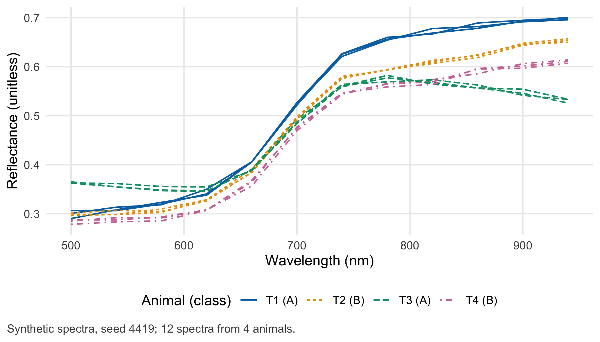
The next block runs on its own in a fresh R session. It generates synthetic reflectance spectra for the same IDs T1 to T4 and classifies them with a one-nearest-neighbour model (class::knn, Venables and Ripley (2002); method background in Methods in R: k-Nearest Neighbours Classification). Each animal has its own level and slope of reflectance (an individual “signature”), and class B adds a weak dip in the near infrared. These spectra are an assumption made for teaching: the animal signature is deliberately stronger than the class signal. All results are stored with the prefix knn_, so they cannot be confused with the hand calculation.
library(class)
set.seed(4419)  # own seed: this block does not depend on earlier chunks

knn_make_spectra <- function(class_effect = 0.03, ids = c("T1", "T2", "T3", "T4"),
                             classes = c("A", "B", "A", "B"), n_per_animal = 3,
                             animal_sd = 0.05, noise_sd = 0.004) {
  wl <- seq(500, 940, by = 40)                                # wavelength in nm
  base <- 0.30 + 0.30 / (1 + exp(-(wl - 690) / 25))          # common tissue curve (reflectance, 0-1)
  rows <- list()
  for (i in seq_along(ids)) {
    level <- rnorm(1, 0, animal_sd)                          # animal-specific offset
    slope <- rnorm(1, 0, animal_sd)                          # animal-specific tilt
    dip <- if (classes[i] == "B") class_effect * exp(-((wl - 800) / 70)^2) else 0
    for (s in seq_len(n_per_animal)) {
      refl <- base + level + slope * (wl - 720) / 220 - dip + rnorm(length(wl), 0, noise_sd)
      rows[[length(rows) + 1]] <- data.frame(id = ids[i], class = classes[i], spectrum = s,
                                             wavelength_nm = wl, reflectance = refl)
    }
  }
  do.call(rbind, rows)
}
knn_to_wide <- function(long) {
  w <- reshape(long, idvar = c("id", "class", "spectrum"), timevar = "wavelength_nm", direction = "wide")
  rownames(w) <- NULL
  w
}
# 1-NN prediction; optional: columns missing at test time are replaced by training means
knn_predict <- function(wide, train, test, available = NULL) {
  X <- as.matrix(wide[, grep("^reflectance", names(wide))])
  if (!is.null(available)) {
    missing_cols <- setdiff(seq_len(ncol(X)), available)
    X[test, missing_cols] <- matrix(colMeans(X[train, missing_cols, drop = FALSE]),
                                    sum(test), length(missing_cols), byrow = TRUE)
  }
  as.character(knn(X[train, , drop = FALSE], X[test, , drop = FALSE],
                   cl = factor(wide$class[train]), k = 1))
}
knn_long <- knn_make_spectra()
knn_wide <- knn_to_wide(knn_long)

# image-wise split: spectra 1-2 train, spectrum 3 test
img_train <- knn_wide$spectrum %in% 1:2
img_test  <- knn_wide$spectrum == 3
knn_img_pred <- knn_predict(knn_wide, img_train, img_test)
knn_img_correct <- sum(knn_img_pred == knn_wide$class[img_test])

# animal-wise two-fold group split (same folds as the split plan)
knn_fold <- c(T1 = 2, T2 = 2, T3 = 1, T4 = 1)[knn_wide$id]
knn_ani <- do.call(rbind, lapply(1:2, function(f) {
  tr <- knn_fold != f; te <- knn_fold == f
  stopifnot(length(intersect(unique(knn_wide$id[tr]), unique(knn_wide$id[te]))) == 0)
  data.frame(fold = f, id = knn_wide$id[te], class = knn_wide$class[te],
             pred = knn_predict(knn_wide, tr, te))
}))
knn_ani_spectra <- sum(knn_ani$pred == knn_ani$class)
# animal-level vote: the majority class of an animal's three spectra
knn_votes <- aggregate(pred ~ id + class, knn_ani, function(p) names(which.max(table(p))))
knn_ani_animals <- sum(knn_votes$pred == knn_votes$class)

knn_votes
#> id class pred
#> 1 T1 A B
#> 2 T3 A B
#> 3 T2 B B
#> 4 T4 B Bc(image_wise = knn_img_correct, animal_wise_spectra = knn_ani_spectra, animal_wise_animals = knn_ani_animals)#> image_wise animal_wise_spectra animal_wise_animals
#> 4 6 2stopifnot(knn_img_correct == 4) # recognition of known animals
stopifnot(nrow(knn_ani) == 12, nrow(knn_votes) == 4) # every animal tested once; denominator 4 animals
stopifnot(knn_ani_spectra == 6, knn_ani_animals == 2, all(knn_ani$pred == "B")) # reference values for this seedThe nearest-neighbour model gets 4 of 4 spectra right in the image-wise split, because the nearest spectrum is almost always another spectrum of the same animal. In the two-fold animal-wise split it gets 6 of 12 spectra and 2 of 4 animals right; in this draw it assigned class B to every test spectrum, so the hits on the two B animals say nothing about the class signal. Unlike the hand calculation, these values come from one random draw; the stopifnot() line records them as reference values for seed 4419, not as properties of the method. The independent denominator is four animals.
19.3.6 Variation between independent animals
One draw of four animals is a single experiment. To see how much an animal-wise result can vary, the next block draws 200 new synthetic cohorts of four animals with the same generator and repeats both tests. This is the step from “one number” to “the spread between independent sets of animals”.
knn_repeat <- function(class_effect, R = 200, available = NULL) {
  res <- replicate(R, {
    w <- knn_to_wide(knn_make_spectra(class_effect = class_effect))
    tr_img <- w$spectrum %in% 1:2; te_img <- w$spectrum == 3
    img <- mean(knn_predict(w, tr_img, te_img, available) == w$class[te_img])
    fold <- c(T1 = 2, T2 = 2, T3 = 1, T4 = 1)[w$id]
    te <- do.call(rbind, lapply(1:2, function(f)
      data.frame(id = w$id[fold == f], class = w$class[fold == f],
                 pred = knn_predict(w, fold != f, fold == f, available))))
    votes <- aggregate(pred ~ id + class, te, function(p) names(which.max(table(p))))
    c(image_wise = img, animal_wise = mean(votes$pred == votes$class))
  })
  t(res)
}
set.seed(4420)
knn_weak <- knn_repeat(class_effect = 0.03)
knn_summary <- data.frame(
  test = c("Image-wise (spectra)", "Animal-wise (animals)"),
  mean = colMeans(knn_weak),
  p05 = apply(knn_weak, 2, quantile, 0.05),
  p95 = apply(knn_weak, 2, quantile, 0.95),
  share_cohorts_at_or_below_half = colMeans(knn_weak <= 0.5)
)
stopifnot(knn_summary$mean[1] > 0.95, knn_summary$mean[2] < 0.7)
knitr::kable(knn_summary, digits = 2, row.names = FALSE,
col.names = c("Test", "Mean accuracy", "5th percentile", "95th percentile", "Cohorts with accuracy ≤ 0.5"))| Test | Mean accuracy | 5th percentile | 95th percentile | Cohorts with accuracy ≤ 0.5 |
|---|---|---|---|---|
| Image-wise (spectra) | 1.00 | 1 | 1 | 0.00 |
| Animal-wise (animals) | 0.52 | 0 | 1 | 0.67 |
Over 200 cohorts the image-wise accuracy stays close to 1 (mean 1.00), while the animal-wise accuracy has a mean of 0.52 and ranges from 0.00 to 1.00 (5th to 95th percentile). In 67% of cohorts the animal-wise result is no better than guessing. The image-wise number is high and stable for the wrong reason.
# leave-one-animal-out on the same kind of cohorts: one fold per animal
set.seed(4422)
knn_loao <- replicate(200, {
  w <- knn_to_wide(knn_make_spectra(class_effect = 0.03))
  mean(sapply(unique(w$id), function(a) {
    p <- knn_predict(w, w$id != a, w$id == a)
    names(which.max(table(p))) == w$class[w$id == a][1]
  }))
})
round(mean(knn_loao), 2)
#> [1] 0.36stopifnot(mean(knn_loao) < 0.5)
WarningCommon mistake
Leave-one-animal-out looks like the strictest split, but with four animals and two classes it leaves only one animal of the held-out class in training. A nearest-neighbour model is then pulled towards the other class. In the 200 synthetic cohorts above, its mean animal-level accuracy is 0.36, below the 0.5 expected from guessing. Check the class balance of every training fold in the split plan, and report the per-animal table instead of a single percentage.
19.3.7 Deepening: a missing modality as a stress test
Many hyperspectral systems combine a visible-range and a near-infrared sensor. Suppose the target centre has only the visible sensor (500–660 nm). A stress test asks what happens when the near-infrared part is missing at test time and is replaced by the training mean, which is a common default in software pipelines. To make the effect visible, the class signal is set strong (class_effect = 0.3), so that the model would work if both sensors were available.
set.seed(4421)
knn_strong <- knn_repeat(class_effect = 0.30)
set.seed(4421)
knn_strong_vis <- knn_repeat(class_effect = 0.30, available = 1:5)  # only 500-660 nm at test time
knn_stress <- rbind(both_sensors = colMeans(knn_strong), visible_only = colMeans(knn_strong_vis))
round(knn_stress, 2)
#> image_wise animal_wise
#> both_sensors 1.00 0.93
#> visible_only 0.63 0.47stopifnot(knn_stress["visible_only", "animal_wise"] < knn_stress["both_sensors", "animal_wise"])With both sensors, the animal-wise accuracy is 0.93; with the near-infrared part missing it drops to 0.47, because the class information sits in the part that is missing. The image-wise accuracy falls as well (to 0.63), since the replaced columns also carried part of each animal’s signature. A stress test of this kind does not replace an external validation at the new centre. It shows before the study which missing input would make the claim collapse, and it forces the team to decide in advance what the system should do when an input is absent: stop, warn, or fall back to the standard assessment.
NoteOther implementation: Python/scikit-learn
Original implementation. GroupKFold in scikit-learn (Pedregosa et al. 2011), version 1.9.1 of the stable documentation (accessed 8 November 2026): GroupKFold. With groups set to the animal ID, each animal appears in exactly one test fold; LeaveOneGroupOut is the variant with one animal per fold.
Concrete advantage. When an imaging model already lives in a Python pipeline with preprocessing and network weights, the group split can sit inside the same pipeline object, so every preprocessing step is fitted within the training fold only.
What must be identical for a fair comparison. The input table (data/b19-spectra.csv), the group column (id), the fold assignment (import fold_animalwise instead of letting each language form its own folds: GroupKFold orders groups arbitrarily and, since version 1.6, can shuffle them), the metric unit (spectrum or animal), k = 1 with Euclidean distance, and the tie rule (class::knn breaks voting ties at random; with continuous spectra and k = 1, ties are practically absent). Tolerance: identical predicted classes.
Shared target value. Zero shared IDs between training and test in every fold. The order of folds may differ.
Status. Conceptual comparison, not executed.
19.4 Counter-check
Change one assumption: make the class signal ten times stronger (class_effect from 0.03 to 0.30). Before you run the block, predict the direction for each test. Will the image-wise accuracy rise, fall or stay the same? And the animal-wise accuracy?
knn_compare <- rbind(weak_signal = colMeans(knn_weak), strong_signal = colMeans(knn_strong))
round(knn_compare, 2)
#> image_wise animal_wise
#> weak_signal 1 0.52
#> strong_signal 1 0.93stopifnot(knn_compare["strong_signal", "animal_wise"] > knn_compare["weak_signal", "animal_wise"],
abs(knn_compare["strong_signal", "image_wise"] - knn_compare["weak_signal", "image_wise"]) < 0.05)The image-wise accuracy is practically unchanged (1.00 and 1.00), whereas the animal-wise accuracy rises from 0.52 to 0.93. The image-wise test gives the same answer whether or not there is anything to learn about the classes. A test that cannot tell these two situations apart cannot support a claim about new animals.
19.5 Consequences for patients and operations
Ethics and the 3Rs. An uninformative test design wastes animals even when few are used. Reduction under the 3Rs means minimising the number of animals consistent with the scientific aims, and the NC3Rs stress that this depends on appropriately designed and analysed studies (NC3Rs 2026). Measuring many spectra per animal can maximise the information gathered per animal, which also counts as reduction, but it does not add independent animals; the experimental unit has to be fixed before the experiment. ARRIVE 2.0 asks authors to state the experimental unit (Essential 10, item 1b) and to discuss generalisability and translation (item 18) (Percie du Sert et al. 2020). For patients, the stake is indirect but real: a feasibility study justified by a recognition test asks participants for time, measurements and possibly images, on a premise that was never tested. The fair sentence in an application is the one that names the tested case.
Regulation. Not touched while the classifier is a research tool. It becomes relevant once a medical intended purpose is stated, for example “supports the assessment of tissue perfusion in patients”; then the questions of Chapter 22 apply, and the evidence must refer to the intended population and setting. A test on known animals is not clinical evidence for any intended purpose.
Data protection. Animal spectra are not personal data. The question changes as soon as patient images are collected for the next study; the data flow, the legal basis for health data and the deletion point are treated in Chapter 23.
Security and traceability. The claim “zero shared IDs” is only as good as the record of which animals were in which fold. Keep the split plan, the fold file and the model version together and under version control (Chapter 4, Chapter 24); a model trained later on “all available data” silently changes which animals are new.
19.6 Look up and transfer
- Reviewer question: Which unit is new in your test set, how many of these units are there, and is the result reported per unit? Please provide the split plan with the number of shared IDs per fold.
- Self-test: A team measures six pigs (three of each class) in two laboratories: pigs 1–4 in laboratory 1, pigs 5–6 in laboratory 2, with 40 spectra per pig. A random 80/20 split of all 240 spectra gives 98% accuracy on 48 test spectra. (a) Which claim does this result support? (b) What is the independent denominator for a claim about new pigs?
- Propose a split for a claim about a new laboratory and say what its denominator would be.
TipAnswer
- Recognition of further spectra from the six known pigs: with 40 spectra per pig, almost every test spectrum has spectra of the same pig in training. (b) The number of pigs in the test folds; with a group split over all six pigs, at most six, and per fold far fewer. Reporting “48 test spectra” overstates the information. (c) Develop in laboratory 1 (pigs 1–4) and test in laboratory 2 (pigs 5–6). The denominator is two pigs, so the only possible results are 0/2, 1/2 and 2/2; check first that laboratory 2 contains both classes. The honest conclusion is that the data cannot support a claim about new laboratories, and that the next study needs more animals or a second external site, not more spectra per animal.
- Annotated sources:
- Justice et al. (1999) distinguish reproducibility from transportability and give the hierarchy of historical, geographic, methodological and spectrum generalisability behind Table 19.1.
- Debray et al. (2015) show how to interpret an external validation in light of case-mix differences between development and validation samples.
- Roberts et al. (2017) explain why random cross-validation underestimates error in clustered data and how to block by group, time or space.
- Kapoor and Narayanan (2023) survey data leakage across 17 fields and give a taxonomy of leak types.
- Zech et al. (2018) document that an imaging model could recognise the hospital system of a radiograph, a measurement-procedure confounder.
- Seok et al. (2013) and Takao and Miyakawa (2015) reach opposite conclusions about mouse–human similarity after trauma and inflammation from the same data, which illustrates that “species similarity” depends on analysis choices.
- Percie du Sert et al. (2020) (ARRIVE 2.0) and NC3Rs (2026) (3Rs) frame the experimental unit and the justification of animal numbers.
- Venables and Ripley (2002) is the reference for the
classpackage andknn(); Pedregosa et al. (2011) for scikit-learn.
The chapter is required reading for W4, where learners split several recordings per animal image-wise and animal-wise and check the ID intersection in R. In W6 the split plan becomes the template for “the next test on another cohort, time or species”, and in W8 groups defend which new case their model refers to.
19.7 Further reading
- Chapter 10 for the hyperspectral measurement chain and why pixel, image, animal and person are different units.
- Chapter 5 for baselines and the order of preprocessing, tuning and testing that the group split must respect.
- Chapter 20 for what happens after a successful external test: shadow operation, drift and monitoring.
- Chapter 27 for reporting the split plan and the tested new case in a model passport.
- Methods in R: Cross-Validation and Nested Cross-Validation for the general resampling schemes.
- Methods in R cheat sheet: External validation for a one-page checklist.
- CTTIR Courses, Course 4, Week 1 Session 1: Cross-validation, nested CV, bootstrap .632+ for a hands-on lab on resampling.
- Methods in R: ARRIVE reporting template for writing up the animal study.