R. Heller · Date: 2026-01-11 · Last changed: 2026-11-09
NoteAt a glance
Guiding question: How does a segmentation decision change the biological conclusion? For: researchers in pathology and translational immunology, doctoral researchers who analyse multiplex tissue images, and reviewers of spatial analyses. · Prerequisites: the unit of analysis from Chapter 3; the measurement chain and pseudoreplication from Chapter 10. In the course:W4 · What imaging, gait and tissue models measure (tissue station) and W5 · Causal questions, trajectories and phenotypes · Data: synthetic (generated in the chapter) · Core reading time: about 10 minutes
12.1 Case and decision
A research pathologist in a fictitious translational group analyses multiplex immunofluorescence images of soft tissue taken from the fracture site during surgery. Twelve patients are included: six whose fractures healed on schedule and six with delayed healing. The hypothesis for a grant application is that T cells and macrophages are more often in direct contact in delayed healing. The image-analysis pipeline finds nuclei with a pretrained segmentation model and then grows every nucleus outwards by a fixed distance to approximate the cell boundary. The lab’s default is 4 µm; a colleague’s older pipeline used 1 µm. With 4 µm, the share of T cells touching a macrophage is clearly higher in delayed healing, and a test over all T cells gives p < 0.01. With 1 µm, the difference almost disappears. The pathologist has to decide which result goes into the application, and what its sample size is. The first error in this chapter is the segment boundary.
12.2 Core reading
Core reading · recommended reading for W4 (tissue station) · about 10 minutes · ends before ‘Lab’
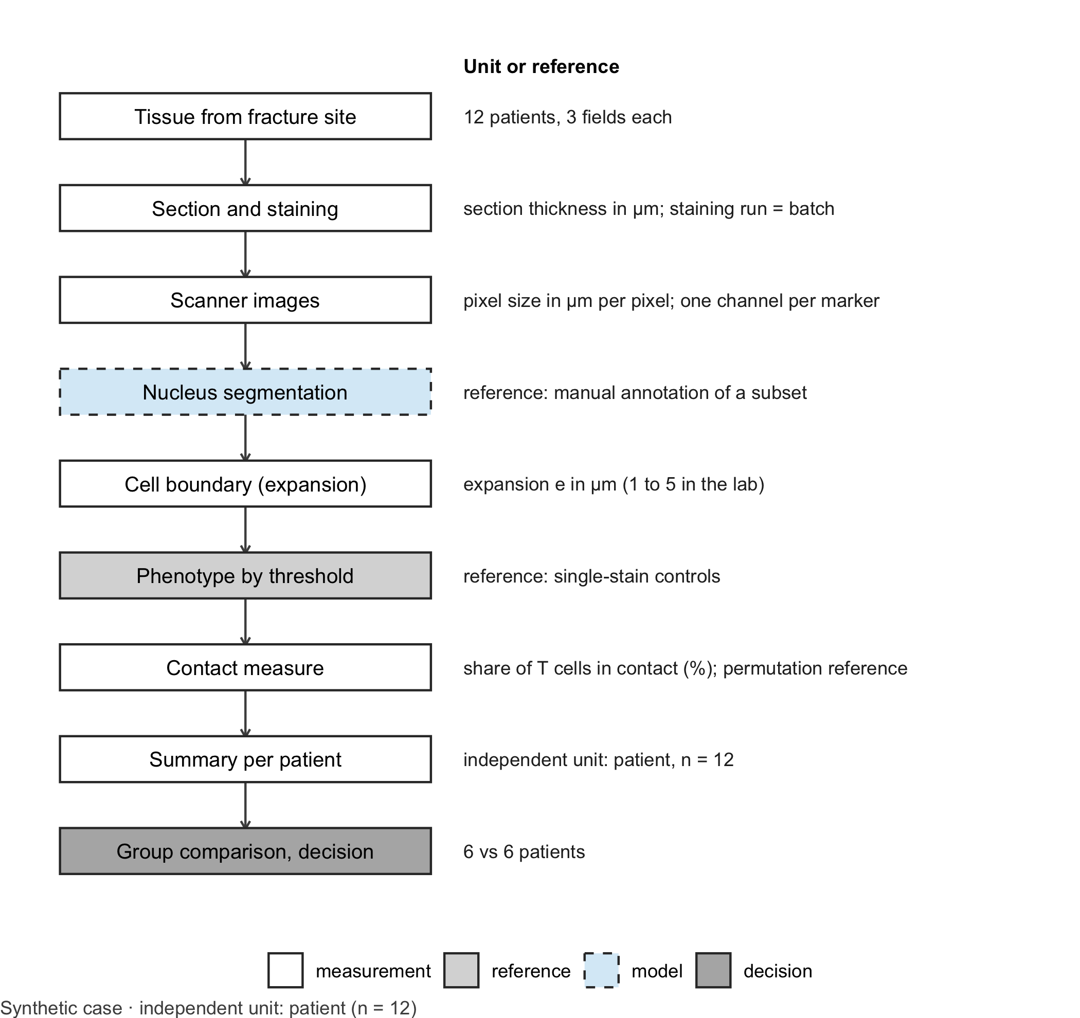
A chain of decisions. A spatial tissue analysis is a long measurement chain (Figure 12.1). Tissue is cut into sections a few micrometres thick and stained with several antibodies at once, for example a nuclear stain, CD3 for T cells and CD68 for macrophages. A scanner records each channel as an image whose pixel size is given in micrometres. A learning model, typically a pretrained network, then segments nuclei (Stringer et al. 2021; Greenwald et al. 2022). Because membranes are harder to see than nuclei, many pipelines approximate each cell by growing its nucleus outwards by a fixed distance. Marker intensities are averaged within this boundary, a threshold assigns a phenotype, and every cell becomes a point with a type. Only then does the neighbourhood analysis begin (Schapiro et al. 2017). Every step contains a parameter, and the boundary expansion is one of the least visible.
Code
library(ggplot2)# Generic drawing of a measurement chain: one box per step, a note per step, dashed border for the learning modeldraw_chain <-function(steps, note_title ="Unit or reference") { steps$y <-rev(seq_len(nrow(steps))) types <-c("measurement", "reference", "model", "decision")ggplot(steps) +geom_segment(data = steps[-nrow(steps), ], aes(x =1, xend =1, y = y -0.24, yend = y -0.76),arrow = grid::arrow(length = grid::unit(0.15, "cm")), colour ="grey30") +geom_tile(aes(x =1, y = y, fill = type, linetype = type), width =1.7, height =0.5,colour ="grey20", linewidth =0.5) +geom_text(aes(x =1, y = y, label = label), size =3.4) +geom_text(aes(x =2.0, y = y, label = note), hjust =0, size =3.1, colour ="grey15") +annotate("text", x =2.0, y =nrow(steps) +0.55, label = note_title, hjust =0, fontface ="bold",size =3.2) +scale_fill_manual(values =c(measurement ="white", reference ="grey85", model ="#D9ECF7",decision ="grey70"), breaks = types, name =NULL) +scale_linetype_manual(values =c(measurement ="solid", reference ="solid", model ="dashed",decision ="solid"), breaks = types, name =NULL) +scale_x_continuous(limits =c(0.1, 4.6)) +scale_y_continuous(limits =c(0.5, nrow(steps) +0.8)) +theme_void(base_size =11) +theme(legend.position ="bottom", plot.caption =element_text(hjust =0, colour ="#4D4D4D"))}chain_b12 <-data.frame(label =c("Tissue from fracture site", "Section and staining", "Scanner images", "Nucleus segmentation","Cell boundary (expansion)", "Phenotype by threshold", "Contact measure", "Summary per patient","Group comparison, decision"),note =c("12 patients, 3 fields each", "section thickness in µm; staining run = batch","pixel size in µm per pixel; one channel per marker", "reference: manual annotation of a subset","expansion e in µm (1 to 5 in the lab)", "reference: single-stain controls","share of T cells in contact (%); permutation reference", "independent unit: patient, n = 12","6 vs 6 patients"),type =c("measurement", "measurement", "measurement", "model", "measurement", "reference", "measurement","measurement", "decision"))draw_chain(chain_b12) +labs(caption ="Synthetic case · independent unit: patient (n = 12)")
Figure 12.1: Measurement chain for a cell-contact analysis in multiplex tissue images. The dashed box marks the learning model (nucleus segmentation); grey boxes mark the reference and the decision. Units change from micrometres to cell types to shares. Independent unit for the group question: patient (n = 12, six per group). Synthetic case.
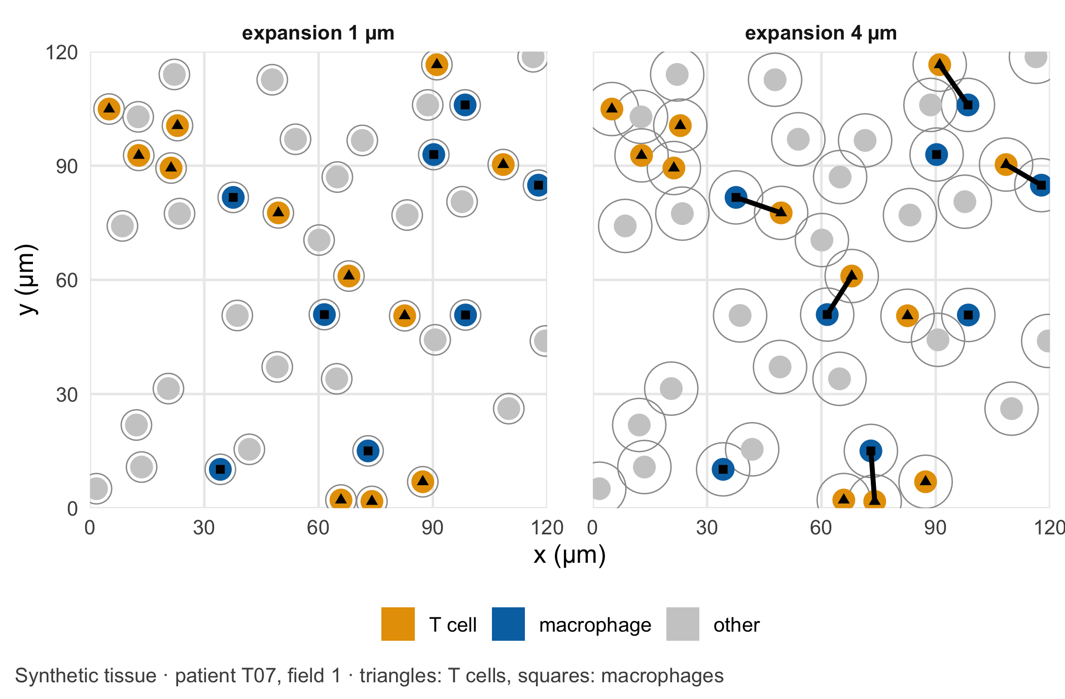
Why the boundary matters. Two cells count as being in contact when their segmented boundaries touch. With nuclei of radius 3 µm and an expansion of \(e\) µm on each side, that happens when the centres are at most \(2(3 + e)\) µm apart: 8 µm for \(e = 1\), 14 µm for \(e = 4\). The area within reach of a cell grows with the square of that distance, so the expansion has a large effect on the number of contacts (Figure 12.2). It has a larger effect where cells are packed more densely. In the synthetic data, tissue from delayed healing contains more cells per square millimetre. A wider boundary therefore produces more chance contacts there, even though the T cells and macrophages are placed without any attraction to each other. The key assumption is that a contact between segmented boundaries reflects a contact between real cells, to the same degree in both groups. Denser tissue, thicker sections or a different staining run can each break this assumption for one group only.
Code
# Choose the 120 µm x 120 µm detail of patient T07, field 1, that contains the most contacts at 4 µmfield_t07 <- cells[cells$patient =="T07"& cells$field ==1, ]count_links <-function(w, e) { t_idx <-which(w$type =="T cell"); m_idx <-which(w$type =="macrophage")if (length(t_idx) ==0||length(m_idx) ==0) return(0) g <-expand.grid(t = t_idx, m = m_idx)sum(sqrt((w$x[g$t] - w$x[g$m])^2+ (w$y[g$t] - w$y[g$m])^2) <=2* (nucleus_radius + e))}origins <-expand.grid(x0 =seq(0, field_size -120, by =20), y0 =seq(0, field_size -120, by =20))origins$links <-apply(origins, 1, function(o) count_links( field_t07[field_t07$x >= o[1] & field_t07$x < o[1] +120& field_t07$y >= o[2] & field_t07$y < o[2] +120, ], 4))best <- origins[which.max(origins$links), ]window <- field_t07[field_t07$x >= best$x0 & field_t07$x < best$x0 +120& field_t07$y >= best$y0 & field_t07$y < best$y0 +120, ]window$x <- window$x - best$x0 # local coordinates of the detailwindow$y <- window$y - best$y0circle <-function(x, y, r, id) { a <-seq(0, 2* pi, length.out =41)data.frame(id = id, x = x + r *cos(a), y = y + r *sin(a))}panels <-lapply(c(1, 4), function(e) { label <-paste0("expansion ", e, " µm") outlines <-do.call(rbind, lapply(seq_len(nrow(window)), function(k)circle(window$x[k], window$y[k], nucleus_radius + e, k))) nuclei <-do.call(rbind, lapply(seq_len(nrow(window)), function(k)cbind(circle(window$x[k], window$y[k], nucleus_radius, k), type = window$type[k]))) t_idx <-which(window$type =="T cell"); m_idx <-which(window$type =="macrophage") pairs <-expand.grid(t = t_idx, m = m_idx) pairs <- pairs[sqrt((window$x[pairs$t] - window$x[pairs$m])^2+ (window$y[pairs$t] - window$y[pairs$m])^2) <=2* (nucleus_radius + e), ] links <-data.frame(x = window$x[pairs$t], y = window$y[pairs$t], xend = window$x[pairs$m],yend = window$y[pairs$m])list(outlines =cbind(outlines, panel = label), nuclei =cbind(nuclei, panel = label),links =if (nrow(links) >0) cbind(links, panel = label) elseNULL,centres =cbind(window, panel = label))})pick <-function(part) do.call(rbind, lapply(panels, `[[`, part))type_levels <-c("T cell", "macrophage", "other")centres <-pick("centres"); centres$type <-factor(centres$type, levels = type_levels)nuclei <-pick("nuclei"); nuclei$type <-factor(nuclei$type, levels = type_levels)ggplot() +geom_polygon(data =pick("outlines"), aes(x, y, group = id), fill =NA, colour ="grey60", linewidth =0.3) +geom_polygon(data = nuclei, aes(x, y, group = id, fill = type), colour =NA) +geom_segment(data =pick("links"), aes(x, y, xend = xend, yend = yend), linewidth =1.1) +geom_point(data = centres[centres$type !="other", ], aes(x, y, shape = type), size =1.6, colour ="black") +facet_wrap(~ panel) +scale_fill_manual(values =c("T cell"=unname(cdsr_colours["orange"]),macrophage =unname(cdsr_colours["blue"]), other ="grey80"), name =NULL) +scale_shape_manual(values =c("T cell"=17, macrophage =15), name =NULL) +guides(shape ="none") +# triangles = T cells, squares = macrophages (see caption)coord_equal(xlim =c(0, 120), ylim =c(0, 120), expand =FALSE) +labs(x ="x (µm)", y ="y (µm)",caption ="Synthetic tissue · patient T07, field 1 · triangles: T cells, squares: macrophages") +theme_cdsr() +theme(panel.spacing = grid::unit(1.5, "lines"))
Figure 12.2: A 120 µm × 120 µm detail of one synthetic field of view from a patient with delayed healing, chosen as the detail with the most contacts at 4 µm. Filled discs: nuclei (radius 3 µm; triangles mark T cells, squares macrophages); grey outlines: cell boundaries after expansion by 1 µm (left) or 4 µm (right); thick lines: T cell–macrophage pairs counted as in contact. Unit: µm. Synthetic data; the independent unit for the study is the patient (n = 12).
Units and the learning step. The units change several times along the chain. Section thickness and distances are micrometres; positions in the image are pixels and become micrometres only through the scanner’s pixel size; cell density is given in cells per square millimetre; the contact measure is a share of T cells. Confusing pixels with micrometres is a silent error, because every number still looks plausible. The learning model sits at the segmentation step. It was trained on other images, often of other tissues and stains. In dense infiltrates, touching nuclei can be merged into one cell or split into two, and that changes cell counts and contacts precisely in the group with the higher density. The segmentation model therefore needs the same scrutiny as the expansion parameter that follows it: its name, version and weights belong in the methods, and its errors should be checked in both groups separately.
What counts as a reference. Each step needs its own check. Segmentation is checked against a pathologist’s manual annotation of a subset of fields, made without knowing the patient’s group. Phenotype thresholds are checked with single-stain controls. For the contact measure itself, the natural reference is what density alone would produce: if the cell types are shuffled at random among the same positions, how often would a T cell touch a macrophage? Comparing the observed share with this permutation expectation separates a specific neighbourhood preference from simple crowding (Schapiro et al. 2017).
Two pipelines, two conclusions. The colleague’s 1 µm and the lab’s 4 µm are both defensible defaults. Neither is right in itself; which one approximates real cell boundaries is an empirical question for the manual reference above. What is not defensible is choosing between them after seeing which gives the larger group difference. The expansion belongs in the analysis plan, fixed after a blinded check against manual boundaries, and the results for a range of expansions belong in the supplement as a sensitivity analysis.
Count patients, not cells. The study images tens of thousands of cells, but the independent unit is the patient. Cells from the same patient share genetics, treatment, surgery and staining; they are pseudoreplicates (Zimmerman et al. 2021). Tests that treat every cell as independent produce false discoveries even in the absence of a biological difference (Squair et al. 2021). Two further pitfalls sit at the edges of the chain. Cells near the border of a field of view have neighbours outside the image that are not counted, which lowers their apparent number of contacts; spatial statistics handle this with edge corrections (Baddeley and Turner 2005). And if the two groups were stained in different runs, a batch effect in staining intensity can shift phenotypes in one group only (Leek et al. 2010), the same structure as the lamp in Chapter 10.
Question for the workshop: Which number would you report as the sample size for the contact comparison, and which single additional analysis would show whether more contacts in delayed healing mean more than more cells?
12.3 Lab
The lab generates twelve fictitious patients with three fields of view each, varies the boundary expansion, recomputes the contact share, compares it with a permutation reference and condenses everything per patient. In the synthetic truth there is no attraction between T cells and macrophages; only the cell density differs between the groups.
Step 1 – the synthetic tissue. The cells were already placed in a hidden chunk of the core reading, because the figure there needs them. Its code is repeated here without being run again: nucleus centres at least 7 µm apart (a simple hard-core process), 15% T cells, 15% macrophages and 70% other cells, assigned at random, and a higher cell density in delayed healing.
# Synthetic tissue: positions and cell types (the lab shows and checks this code step by step)field_size <-500# field of view, µm per sidenucleus_radius <-3# µmmin_gap <-7# minimum distance between nucleus centres, µmplace_cells <-function(n, size = field_size, min_dist = min_gap) { x <-numeric(0); y <-numeric(0); tries <-0while (length(x) < n && tries <50* n) { tries <- tries +1 cx <-runif(1, 0, size); cy <-runif(1, 0, size)if (length(x) ==0||min((x - cx)^2+ (y - cy)^2) >= min_dist^2) { x <-c(x, cx); y <-c(y, cy) } }data.frame(x = x, y = y)}patients <-data.frame(patient =sprintf("T%02d", 1:12), group =rep(c("uneventful", "delayed"), each =6))patients$density <-ifelse(patients$group =="delayed", rnorm(12, 3000, 300), rnorm(12, 2200, 250))cell_list <-list()for (i in1:12) for (f in1:3) { n <-rpois(1, patients$density[i] * (field_size /1000)^2) p <-place_cells(n) p$type <-sample(c("T cell", "macrophage", "other"), nrow(p), replace =TRUE, prob =c(0.15, 0.15, 0.70)) p$patient <- patients$patient[i]; p$group <- patients$group[i]; p$field <- f cell_list[[length(cell_list) +1]] <- p}cells <-do.call(rbind, cell_list)
Then we check the design.
cells_per_field <-aggregate(x ~ patient + group + field, data = cells, FUN = length)names(cells_per_field)[4] <-"cells"density_per_patient <-aggregate(cells ~ patient + group, data = cells_per_field, FUN = mean)density_per_patient$cells_per_mm2 <- density_per_patient$cells / (field_size /1000)^2aggregate(cells_per_mm2 ~ group, data = density_per_patient, FUN = mean)
Step 2 – contacts for a given boundary. For each field we list all pairs of cells whose centres are close enough to touch at the largest expansion. The contact share for any expansion is then a filter on this list.
expansions <-1:5# boundary expansion in µmmax_reach <-2* (nucleus_radius +max(expansions)) # centre distance for contact at 5 µmclose_pairs <-function(d) { D <-as.matrix(dist(d[, c("x", "y")])) idx <-which(D <= max_reach &upper.tri(D), arr.ind =TRUE)data.frame(i = idx[, 1], j = idx[, 2], distance = D[idx])}# Share of T cells with at least one macrophage contact; 'edge' drops T cells whose reach crosses the bordercontact_count <-function(d, pairs, e, types = d$type, edge =FALSE) { reach <-2* (nucleus_radius + e) p <- pairs[pairs$distance <= reach, ] t_cells <-which(types =="T cell")if (edge) t_cells <- t_cells[d$x[t_cells] > reach & d$x[t_cells] < field_size - reach & d$y[t_cells] > reach & d$y[t_cells] < field_size - reach] touching <-c(p$i[types[p$j] =="macrophage"], p$j[types[p$i] =="macrophage"])c(t_cells =length(t_cells), in_contact =sum(t_cells %in% touching))}
Step 3 – shift the boundary and build the permutation reference. For every field and expansion we record the observed contacts, the contacts after excluding T cells near the border, and the share expected if the cell types were shuffled at random among the same positions (100 permutations per field).
set.seed(2212)field_keys <-unique(cells[, c("patient", "group", "field")])per_field <-do.call(rbind, lapply(seq_len(nrow(field_keys)), function(k) { d <- cells[cells$patient == field_keys$patient[k] & cells$field == field_keys$field[k], ] pairs <-close_pairs(d)do.call(rbind, lapply(expansions, function(e) { observed <-contact_count(d, pairs, e) inner <-contact_count(d, pairs, e, edge =TRUE) shuffled <-replicate(100, { s <-contact_count(d, pairs, e, types =sample(d$type)); s[2] / s[1] })data.frame(field_keys[k, ], expansion = e, t_cells = observed[1], in_contact = observed[2],t_cells_inner = inner[1], in_contact_inner = inner[2], expected_share =mean(shuffled)) }))}))# Condense per patient: pooled counts over the three fieldsper_patient <-aggregate(cbind(t_cells, in_contact, t_cells_inner, in_contact_inner) ~ patient + group + expansion,data = per_field, FUN = sum)per_patient <-merge(per_patient, aggregate(expected_share ~ patient + expansion, data = per_field, FUN = mean))per_patient$share <- per_patient$in_contact / per_patient$t_cellsper_patient$share_inner <- per_patient$in_contact_inner / per_patient$t_cells_innerper_patient$ratio <- per_patient$share / per_patient$expected_share# Contacts can only increase with a wider boundary, for every patientmonotone <-tapply(seq_len(nrow(per_patient)), per_patient$patient, function(k)all(diff(per_patient$share[k][order(per_patient$expansion[k])]) >=0))stopifnot(all(monotone))round(aggregate(cbind(share, expected_share, ratio) ~ group + expansion, data = per_patient, FUN = mean)[, -1], 3)
Step 4 – the same question at two levels. For the colleague’s 1 µm and the default 4 µm we test the group difference once over all T cells, as if they were independent, and once with one value per patient.
compare_levels <-function(e) { d <- per_patient[per_patient$expansion == e, ] pooled <-aggregate(cbind(in_contact, t_cells) ~ group, data = d, FUN = sum)data.frame(expansion_um = e,share_delayed =mean(d$share[d$group =="delayed"]),share_uneventful =mean(d$share[d$group =="uneventful"]),n_t_cells =sum(d$t_cells),p_cells =prop.test(pooled$in_contact, pooled$t_cells)$p.value, # every T cell as a unitn_patients =nrow(d),p_patients =t.test(share ~ group, data = d)$p.value, # one value per patientp_ratio =t.test(ratio ~ group, data = d)$p.value) # density-adjusted}levels_test <-rbind(compare_levels(1), compare_levels(4))levels_test
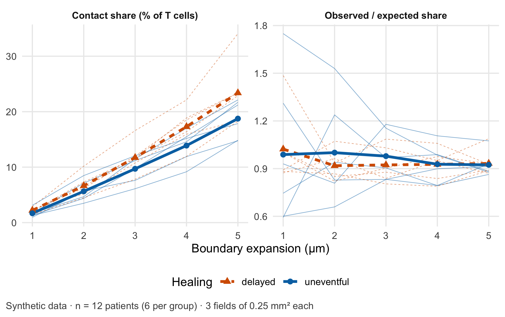
At 1 µm the groups differ by 0.5 percentage points; at 4 µm by 3.4 points. Only the boundary changed. The test over 3,478 T cells reports p = 0.0032 at 4 µm; the test over 12 patients reports p = 0.092. The density-adjusted ratio, observed divided by expected share, is close to 1 in both groups (p = 0.99): the extra contacts in delayed healing are what crowding alone produces. Figure 12.3 shows the whole range of expansions.
Code
long <-rbind(data.frame(per_patient[, c("patient", "group", "expansion")], value =100* per_patient$share,panel ="Contact share (% of T cells)"),data.frame(per_patient[, c("patient", "group", "expansion")], value = per_patient$ratio,panel ="Observed / expected share"))means <-aggregate(value ~ group + expansion + panel, data = long, FUN = mean)ggplot(long, aes(expansion, value, colour = group, linetype = group)) +geom_line(aes(group = patient), linewidth =0.3, alpha =0.5) +geom_line(data = means, linewidth =1.3) +geom_point(data = means, aes(shape = group), size =2.4) +facet_wrap(~ panel, scales ="free_y") +scale_colour_manual(values =unname(cdsr_colours[c("red", "blue")])) +scale_linetype_manual(values = cdsr_linetypes[c(2, 1)]) +scale_shape_manual(values = cdsr_shapes[c(2, 1)]) +labs(x ="Boundary expansion (µm)", y =NULL, colour ="Healing", linetype ="Healing", shape ="Healing",caption ="Synthetic data · n = 12 patients (6 per group) · 3 fields of 0.25 mm² each") +theme_cdsr()
Figure 12.3: Left: share of T cells in contact with at least one macrophage, per patient (thin lines) and group mean (thick lines), against the boundary expansion in µm. Right: the same share divided by the share expected from random placement of cell types (permutation reference); 1 means no preference beyond density. Synthetic data; independent unit: patient (n = 12, six per group); 3 fields of 500 µm × 500 µm per patient.
WarningCommon mistake
Reporting “n = 3,478 T cells” as the sample size. Cells, fields and pixels are measurements within patients. The sample size for a comparison between groups of patients is the number of patients; the number of cells per patient describes the precision of each patient’s value and belongs next to it.
Step 5 – what condensing per patient loses. Condensing to one share per patient is what makes the test honest, but it discards information that belongs in the report.
Three things disappear in the patient summary. First, precision: the shares rest on between 210 and 452 T cells per patient, so they are not equally reliable. Second, heterogeneity: the three fields of one patient can differ by several percentage points, and a single field with a dense aggregate can dominate. Third, the spatial arrangement itself: where in the tissue the contacts occur, for example near vessels or at the fracture gap, is no longer visible. Reporting the number of T cells and fields per patient, and the range across fields, keeps the loss transparent. Models that keep the cells but treat the patient as the unit, such as generalised linear mixed models, are the next step (Methods in R: glmer: Generalised Mixed Models).
NoteOther implementation: Python with scikit-image and Cellpose
In practice the segmentation runs in Python. scikit-image (0.26.0 in November 2026) provides skimage.segmentation.expand_labels(label_image, distance), which “expands labels in label image by distance pixels without overlapping”, and skimage.measure.regionprops_table for centroids and mean marker intensities (Walt et al. 2014). The distance is given in pixels: at 0.5 µm per pixel, the lab’s 4 µm become 8 pixels, and a pipeline that forgets the conversion silently doubles or halves the boundary. Nuclei are often found with Cellpose (4.2.1 in November 2026), a PyTorch-based generalist model (Stringer et al. 2021; Paszke et al. 2019); its current model uses the first three image channels and was trained on objects of about 7.5 to 120 pixels in diameter, so channel order and pixel size must be documented. The concrete advantage is a tested segmentation of real images, which this lab replaces by synthetic points. For a fair comparison the following must be identical: pixel size, the label image, the expansion in µm, the contact definition (labels that touch after expansion), the field borders and edge rule, and the per-patient aggregation. Because expand_labels stops where two growing cells meet, a third cell between two others can block a contact that the distance rule in this lab would count; the shares should therefore agree closely but not exactly, and the tolerance (for example one percentage point per patient) has to be set beforehand. Status: conceptual comparison, not run.
12.4 Counter-check
Predict first: if T cells whose reach crosses the border of the field are excluded, does the contact share rise or fall, and does the conclusion of the group comparison change?
The border correction raises the share slightly in both groups, because cells at the border lose neighbours that lie outside the image. With 500 µm fields and a reach of 14 µm the effect is small and does not change the patient-level result (p = 0.069). It grows with smaller fields and larger reach. A second counter-check is a thought experiment that the lab has already answered: if both groups had the same cell density, the gap in contact share would shrink towards zero at every expansion, which is what the observed/expected ratio in Figure 12.3 shows.
The checkable measurement assumption of this case is: the boundary expansion, converted to pixels with the scanner’s pixel size, reproduces a pathologist’s manual cell boundaries in a blinded subset of fields of both groups equally well. The plausible failure mode is: a default expansion chosen for sparse tissue creates chance contacts in dense tissue and turns a difference in cellularity into an apparent difference in cell interaction.
12.5 Consequences for patients and operations
A misleading sample size. The most direct harm in this case is a number. “p < 0.01 in more than 3,000 T cells” reads like strong evidence and can secure funding, steer a follow-up study and recruit further patients for tissue donation, all for a difference that crowding explains. The honest statement is “12 patients, six per group, no difference in density-adjusted contacts”. Patients who donate tissue do so on the assumption that their samples are analysed in a way that can answer the question.
Wrong tissue interpretation. If a contact score were later used to classify patients, for example as at risk of delayed healing, the segmentation parameter would decide which patients receive closer follow-up or additional procedures. Software that analyses images of tissue specimens to provide information on a pathological state may fall under the In Vitro Diagnostic Medical Devices Regulation (EU) 2017/746, whose definition covers software intended to be used in vitro for the examination of specimens derived from the human body [European Parliament and Council of the European Union (2017); binding text]. Whether a given tool is such a device depends on its intended purpose; the guidance MDCG 2019-11 Rev. 1 helps with the qualification but is not binding (Medical Device Coordination Group 2025). Chapter 22 works through an IVD vignette.
Data protection. Whole-slide images linked with clinical data are health data. Rare combinations of diagnosis, age and date of surgery can identify a patient even without a name; Chapter 23 and Chapter 26 discuss minimisation and controlled access.
Operations and integrity. The expansion distance, the segmentation model and its version, the pixel size and the phenotype thresholds are part of the result. They belong in the model passport (Chapter 27) and should be stored with a checksum, so that a later re-analysis can show that it used the same parameters (Chapter 24).
12.6 Look up and transfer
Reviewer question: The manuscript reports a significant increase in T cell–macrophage contacts “in 4,812 cells”. How many patients contributed, how was the cell boundary defined and in which unit, and was the contact frequency compared with what cell density alone would produce?
Self-test: A second study uses the same pipeline but images only one field of 250 µm × 250 µm per patient, and the boundary expansion is set to 5 µm. Without computing: will the border effect be larger or smaller than in the lab, will the gap between dense and sparse tissue be larger or smaller, and what is the independent sample size if 20 patients contribute 9,000 T cells?
TipAnswer
The border effect will be larger. A smaller field has more cells near its border relative to its area, and the reach grows to \(2(3 + 5) = 16\) µm, so a larger share of T cells has neighbours outside the image. The gap between dense and sparse tissue will also be larger, because a wider boundary produces more chance contacts where cells are packed more tightly. The independent sample size is 20 patients; the 9,000 T cells are repeated measurements within them. A density-adjusted measure, such as the observed share divided by a permutation expectation, and an edge correction belong in the analysis plan before the data are seen.
Annotated sources:
Schapiro et al. (2017) introduced neighbourhood analysis of multiplexed tissue images against a permutation reference, the idea behind the observed/expected ratio.
Stringer et al. (2021) and Greenwald et al. (2022) describe pretrained segmentation models, the learning step of the chain.
Zimmerman et al. (2021) shows that cells from one individual are pseudoreplicates and that ignoring this inflates type I error.
Squair et al. (2021) demonstrates false discoveries when variation between biological replicates is ignored.
Baddeley and Turner (2005) documents the R tools for spatial point patterns, including edge corrections.
Leek et al. (2010) explains how batch effects can masquerade as biology.
European Parliament and Council of the European Union (2017) and Medical Device Coordination Group (2025) are the binding text and the non-binding guidance for the regulatory paragraph.
12.7 Further reading
Chapter 14 – when a pattern in high-dimensional data is a cluster, a gradient or an artefact.
Chapter 26 – controlled access and minimisation for image data linked to patients.
Chapter 22 – the IVD vignette and how an intended purpose changes the regulatory question.
Baddeley, Adrian, and Rolf Turner. 2005. “Spatstat: An R Package for Analyzing Spatial Point Patterns.”Journal of Statistical Software 12 (6): 1–42. https://doi.org/10.18637/jss.v012.i06.
Greenwald, Noah F., Geneva Miller, Erick Moen, Alex Kong, et al. 2022. “Whole-Cell Segmentation of Tissue Images with Human-Level Performance Using Large-Scale Data Annotation and Deep Learning.”Nature Biotechnology 40 (4): 555–65. https://doi.org/10.1038/s41587-021-01094-0.
Leek, Jeffrey T., Robert B. Scharpf, Héctor Corrada Bravo, David Simcha, et al. 2010. “Tackling the Widespread and Critical Impact of Batch Effects in High-Throughput Data.”Nature Reviews Genetics 11 (10): 733–39. https://doi.org/10.1038/nrg2825.
Schapiro, Denis, Hartland W. Jackson, Swetha Raghuraman, Jana R. Fischer, et al. 2017. “histoCAT: Analysis of Cell Phenotypes and Interactions in Multiplex Image Cytometry Data.”Nature Methods 14 (9): 873–76. https://doi.org/10.1038/nmeth.4391.
Squair, Jordan W., Matthieu Gautier, Claudia Kathe, Mark A. Anderson, et al. 2021. “Confronting False Discoveries in Single-Cell Differential Expression.”Nature Communications 12 (1): 5692. https://doi.org/10.1038/s41467-021-25960-2.
Stringer, Carsen, Tim Wang, Michalis Michaelos, and Marius Pachitariu. 2021. “Cellpose: A Generalist Algorithm for Cellular Segmentation.”Nature Methods 18 (1): 100–106. https://doi.org/10.1038/s41592-020-01018-x.
Walt, Stéfan van der, Johannes L. Schönberger, Juan Nunez-Iglesias, et al. 2014. “Scikit-Image: Image Processing in Python.”PeerJ 2: e453. https://doi.org/10.7717/peerj.453.
Zimmerman, Kip D., Mark A. Espeland, and Carl D. Langefeld. 2021. “A Practical Solution to Pseudoreplication Bias in Single-Cell Studies.”Nature Communications 12 (1): 738. https://doi.org/10.1038/s41467-021-21038-1.