R. Heller · Date: 2026-03-08 · Last changed: 2026-11-09
NoteAt a glance
Guiding question: What separates a biological signal from illumination and device characteristics? For: doctoral researchers and preclinical teams who analyse spectral images, and reviewers of such studies. · Prerequisites: analysis units and denominators from Chapter 3; baseline thinking from Chapter 5. In the course:W4 · What imaging, gait and tissue models measure · Data: synthetic (generated in the chapter; fictitious animals) · Core reading time: about 10 minutes
10.1 Case and decision
A doctoral researcher in a fictitious preclinical group analyses hyperspectral images of skin flaps in eight rats. The question is whether a fictitious substance improves the oxygenation of the flap tip on day 3. The four control animals were imaged in the first week, the four treated animals in the second. Between the two weeks the camera lamp was replaced. The camera records a new white reference at every start-up, but the analysis script still loads the file from the first day. The oxygenation index of the treated animals is clearly higher, and a t-test over all pixels returns a p-value far below 0.001. The supervisor wants to submit an abstract this week. The researcher has to decide whether to report a treatment effect, or first to check the calibration and count how many independent units the study really has. The first error in this chapter is not statistical. It is the light.
10.2 Core reading
Core reading · required for W4 · about 10 minutes · ends before ‘Lab’
What the camera records. A hyperspectral camera stores a cube of numbers: two spatial axes and one spectral axis. Every pixel holds a spectrum, here 101 values from 500 to 1,000 nm in steps of 5 nm. The raw value in each band is a count from the sensor (digital numbers, DN). It is the product of three things: how much light the lamp emits at that wavelength, how much of it the tissue reflects, and how sensitive the sensor is at that wavelength. Only the middle factor is biology (Lu and Fei 2014).
Calibration turns counts into reflectance. Two reference images separate the tissue from the device. A dark reference, taken with the shutter closed, records the sensor’s offset. A white reference, taken of a standard tile that reflects almost all light (here 99%), records lamp and sensor together. The reflectance of a pixel is then \(R(\lambda) = 0.99 \cdot (\text{raw} - \text{dark}) / (\text{white} - \text{dark})\), a dimensionless share between 0 and 1. The key assumption is that the white reference was recorded under the same light as the tissue image. If the lamp changes in between, the division no longer cancels it.
From spectrum to index. Deoxygenated haemoglobin absorbs red light around 660 nm much more strongly than oxygenated haemoglobin, whereas around 800 nm the two absorb similarly. The ratio \(R(660)/R(800)\) therefore rises with oxygenation. Real perfusion parameters are more elaborate and are derived from validated absorption models (Holmer et al. 2018); the index in this chapter is a didactic simplification built on synthetic absorption profiles. A ratio has one useful property: it cancels anything that scales the whole spectrum, such as the distance between camera and tissue. It does not cancel anything that changes the shape of the spectrum.
Two kinds of reference. The word “reference” means two different things in this chapter. The white and dark references are technical references: they turn the number on the screen into a reflectance, and a grey tile of known reflectance can check them at every session. A biological reference answers another question: does the index track tissue oxygenation at all? That would need an independent measurement in the same tissue, for example an invasive oxygen probe or a histological marker of ischaemia, read without knowledge of the index. The synthetic study has no such reference; its absence is recorded as open. Without it, a higher index means “the tissue reflects relatively more red light”, not “the tissue is better oxygenated”. The physical units change along the chain: wavelength in nanometres, raw signal in counts, reflectance as a share between 0 and 1, and the index as a dimensionless ratio. A difference of 0.05 index units has no clinical meaning until a biological reference has given it one.
What went wrong. The replacement lamp is brighter and emits relatively more red light. Brightness alone would not matter for a ratio. The change in colour does: with the old white reference, the reflectance at 660 nm is inflated relative to 800 nm by a factor of 1.117, and so is every index measured in week 2 (synthetic). Because all treated animals were imaged in week 2, lamp and treatment are completely confounded. No statistical model can separate them; only a calibration with the matching white reference can. A gain of about 12% is roughly the difference between the poorly perfused tip and the well perfused base of a flap in the synthetic data, so the artefact is large enough to look like biology.
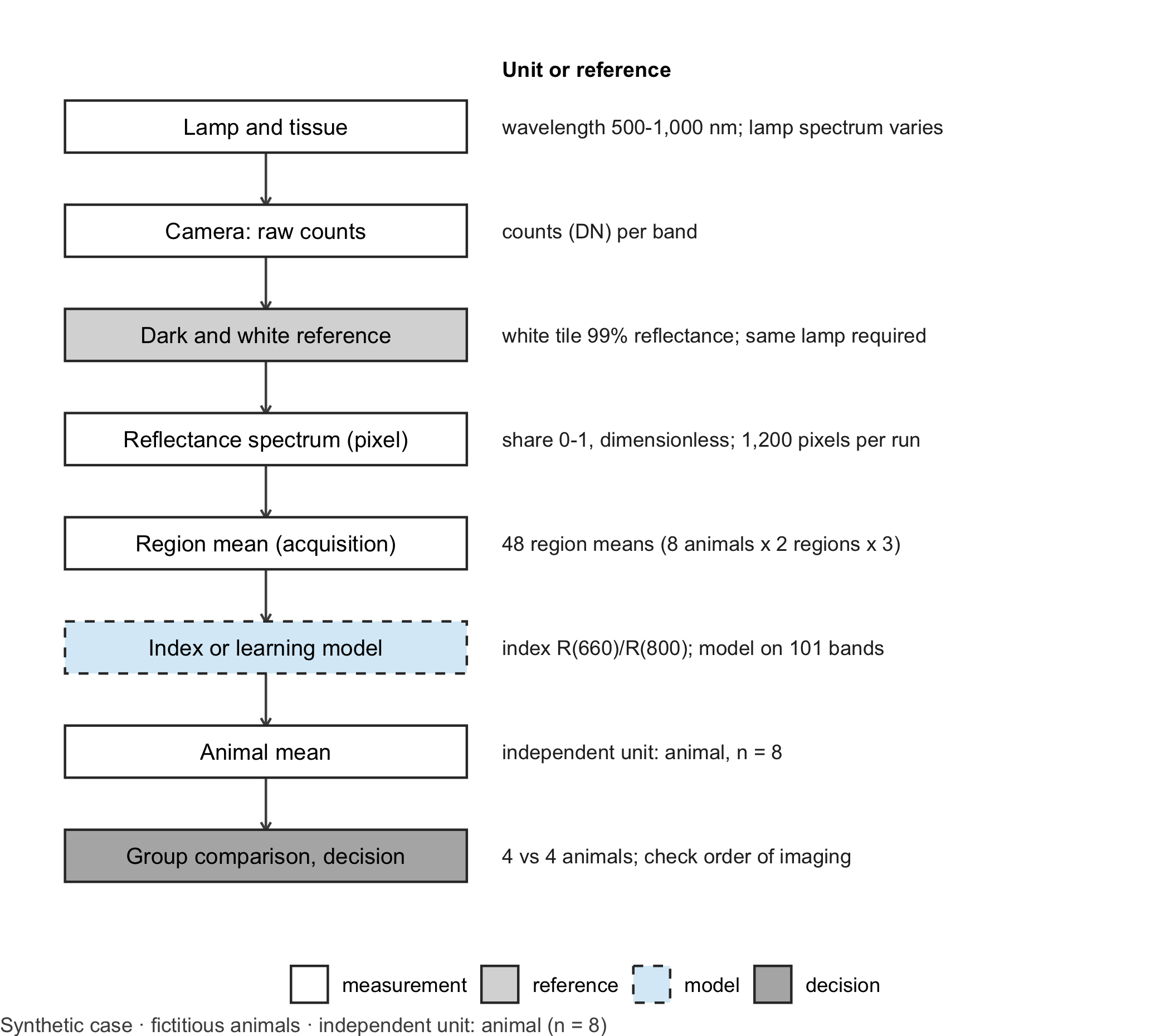
The measurement chain.Figure 10.1 lays out each step from lamp to decision. It marks where the references enter, where the physical unit changes and where a learning model could replace the simple index. Drawing the chain before analysing data is the quickest way to find the step at which a device property can masquerade as a treatment effect.
Code
library(ggplot2)# Generic drawing of a measurement chain: one box per step, a note per step, dashed border for the learning modeldraw_chain <-function(steps, note_title ="Unit or reference") { steps$y <-rev(seq_len(nrow(steps))) types <-c("measurement", "reference", "model", "decision")ggplot(steps) +geom_segment(data = steps[-nrow(steps), ], aes(x =1, xend =1, y = y -0.24, yend = y -0.76),arrow = grid::arrow(length = grid::unit(0.15, "cm")), colour ="grey30") +geom_tile(aes(x =1, y = y, fill = type, linetype = type), width =1.7, height =0.5,colour ="grey20", linewidth =0.5) +geom_text(aes(x =1, y = y, label = label), size =3.4) +geom_text(aes(x =2.0, y = y, label = note), hjust =0, size =3.1, colour ="grey15") +annotate("text", x =2.0, y =nrow(steps) +0.55, label = note_title, hjust =0, fontface ="bold",size =3.2) +scale_fill_manual(values =c(measurement ="white", reference ="grey85", model ="#D9ECF7",decision ="grey70"), breaks = types, name =NULL) +scale_linetype_manual(values =c(measurement ="solid", reference ="solid", model ="dashed",decision ="solid"), breaks = types, name =NULL) +scale_x_continuous(limits =c(0.1, 4.6)) +scale_y_continuous(limits =c(0.5, nrow(steps) +0.8)) +theme_void(base_size =11) +theme(legend.position ="bottom", plot.caption =element_text(hjust =0, colour ="#4D4D4D"))}chain_b10 <-data.frame(label =c("Lamp and tissue", "Camera: raw counts", "Dark and white reference", "Reflectance spectrum (pixel)","Region mean (acquisition)", "Index or learning model", "Animal mean", "Group comparison, decision"),note =c("wavelength 500-1,000 nm; lamp spectrum varies", "counts (DN) per band","white tile 99% reflectance; same lamp required", "share 0-1, dimensionless; 1,200 pixels per run","48 region means (8 animals x 2 regions x 3)", "index R(660)/R(800); model on 101 bands","independent unit: animal, n = 8", "4 vs 4 animals; check order of imaging"),type =c("measurement", "measurement", "reference", "measurement", "measurement", "model", "measurement","decision"))draw_chain(chain_b10) +labs(caption ="Synthetic case · fictitious animals · independent unit: animal (n = 8)")
Figure 10.1: Measurement chain for the hyperspectral case. Each box is one step, the right-hand column gives the unit or the reference at that step. The dashed box marks where a learning model can replace the index. Independent unit for the treatment question: animal (n = 8, four per group). Synthetic case.
Count the units before testing. The study produces many numbers, but few independent ones (Table 10.1). Pixels within one region share the same animal, the same lamp and the same acquisition; they are pseudoreplicates, not replicates (Lazic 2010). The experimental unit is the animal, as the ARRIVE guidelines ask authors to state explicitly (Percie du Sert et al. 2020).
Table 10.1: Analysis levels in the hyperspectral case. Synthetic design; independent unit for the treatment question: animal (n = 8).
Level
Count in the case
What varies at this level
Unit for the treatment test?
Pixel
1,200 (8 × 2 × 3 × 25)
noise, small-scale tissue texture
no
Region in one acquisition
48
positioning, brightness
no
Animal
8 (4 per group)
biology, treatment
yes
Imaging week
2
lamp, calibration file
confounded with group
Where the learning model sits. A classifier trained on full spectra could replace the index in step six of the chain, for instance to tell well and poorly perfused tissue apart. It sits after calibration and inherits every calibration error. It therefore has to be compared with the simple index on new animals, not on new pixels of known animals, and it has to pass the same illumination check.
Question for the workshop: Which single additional image, taken at every imaging session, would have revealed the lamp problem before any animal was analysed, and what value would you expect it to show?
10.3 Lab
The lab simulates the whole chain: synthetic tissue spectra, lamp, sensor, dark and white references, calibration, the index, a grouped test and a comparison of the index with a learning model on new animals. All absorption profiles are synthetic and qualitative; they are not tabulated extinction coefficients.
Step 1 – tissue, lamps and sensor.
wl <-seq(500, 1000, by =5) # wavelengths in nm (101 bands)bump <-function(centre, width) exp(-0.5* ((wl - centre) / width)^2)# Synthetic absorption profiles: deoxygenated absorbs strongly around 660 nm, both are similar near 800 nmabs_deoxy <-1.00*bump(555, 22) +0.32*bump(650, 60) +0.10*bump(760, 14) +0.06abs_oxy <-0.85*bump(542, 11) +0.90*bump(577, 10) +0.05*bump(900, 90) +0.06# Tissue reflectance (share 0-1) for oxygen saturation 'sat', blood volume factor and scattering factortissue_reflectance <-function(sat, blood, scatter =1) { background <- (0.55+0.00025* (wl -500)) * scatter background *exp(-blood * (sat * abs_oxy + (1- sat) * abs_deoxy))}lamp_A <-0.45+0.55* (wl -500) /500# original lamp, rising towards the infraredlamp_B <-1.2* lamp_A * (1+0.25* (800- wl) /300) # replacement: 20% brighter, relatively more redsensor <-0.95-0.45* ((wl -720) /300)^2# relative sensor sensitivityfull_scale <-20000# counts for a perfect reflectordark_level <-300# sensor offset in counts# Raw counts of one spectrum: signal plus offset plus photon noiseraw_counts <-function(reflectance, lamp) { signal <- full_scale * lamp * sensor * reflectance signal + dark_level +rnorm(length(signal), 0, sqrt(signal + dark_level))}# Index of one spectrum (vector) or of every pixel (matrix with one column per pixel)oxygen_index <-function(R) {if (is.matrix(R)) R[wl ==660, ] / R[wl ==800, ] else R[wl ==660] / R[wl ==800]}round(c(poorly_oxygenated =oxygen_index(tissue_reflectance(0.45, 1.5)),well_oxygenated =oxygen_index(tissue_reflectance(0.70, 1.5))), 3)
Step 2 – dark and white references and a check. The white reference is the mean of ten frames of the 99% tile under each lamp. A grey tile with a flat reflectance of 50% serves as a check: after calibration its spectrum must be flat at 0.5 and its index must be 1.00 within a tolerance of ±0.02, set before the study (assumption).
set.seed(1010)lamps <-list(week1 = lamp_A, week2 = lamp_B)white_ref <-lapply(lamps, function(l) rowMeans(sapply(1:10, function(i) raw_counts(rep(0.99, length(wl)), l))))calibrate <-function(raw, white) 0.99* (raw - dark_level) / (white - dark_level)# Grey check tile: mean of 100 pixels, calibrated with the matching and with the stale white referencegrey_tile <-function(week, white) { raw <-sapply(1:100, function(i) raw_counts(rep(0.50, length(wl)), lamps[[week]]))rowMeans(calibrate(raw, white))}check <-data.frame(week =c("week 1", "week 2", "week 2"),white_reference =c("matching", "matching", "stale (week 1)"),mean_reflectance =c(mean(grey_tile(1, white_ref$week1)), mean(grey_tile(2, white_ref$week2)),mean(grey_tile(2, white_ref$week1))),grey_index =c(oxygen_index(grey_tile(1, white_ref$week1)), oxygen_index(grey_tile(2, white_ref$week2)),oxygen_index(grey_tile(2, white_ref$week1))))check$within_tolerance <-abs(check$grey_index -1) <=0.02check
The stale white reference fails the grey check in week 2. The check needs no animal and no statistics.
Step 3 – eight fictitious animals. In the synthetic truth the substance has no effect: both groups draw their oxygen saturation from the same distribution. Each animal has two regions (flap base and flap tip), three acquisitions per region and 25 pixels per region of interest.
set.seed(2018)animals <-data.frame(animal =sprintf("R%02d", 1:8), group =rep(c("control", "treatment"), each =4),week =rep(1:2, each =4))animals$blood <-rnorm(8, 1.5, 0.15) # blood volume factor per animalanimals$scatter <-rnorm(8, 1, 0.05) # scattering factor per animalanimals$sat_base <-rnorm(8, 0.70, 0.03) # no treatment effect in the synthetic truthanimals$sat_tip <- animals$sat_base -rnorm(8, 0.25, 0.03) # the tip is less well perfusedpixel_rows <-list()spectrum_rows <-list()for (a in1:8) for (region inc("base", "tip")) for (acq in1:3) { sat <-if (region =="base") animals$sat_base[a] else animals$sat_tip[a] sat_acq <- sat +rnorm(1, 0, 0.01) # small change between acquisitions brightness <-rnorm(1, 1, 0.05) # distance and angle change the overall level raw <-sapply(1:25, function(p) raw_counts( brightness *tissue_reflectance(sat_acq +rnorm(1, 0, 0.02), animals$blood[a], animals$scatter[a]), lamps[[animals$week[a]]]))for (cal inc("stale", "matching")) { white <-if (cal =="matching") white_ref[[animals$week[a]]] else white_ref$week1 R <-calibrate(raw, white) # 101 bands x 25 pixels info <-data.frame(animal = animals$animal[a], group = animals$group[a], week = animals$week[a],region = region, acquisition = acq, calibration = cal) pixel_rows[[length(pixel_rows) +1]] <-cbind(info, pixel =1:25, index =oxygen_index(R)) spectrum_rows[[length(spectrum_rows) +1]] <-cbind(info, t(rowMeans(R))) }}pixels <-do.call(rbind, pixel_rows)spectra <-do.call(rbind, spectrum_rows)names(spectra)[-(1:6)] <-paste0("nm", wl)spectra$index <- spectra$nm660 / spectra$nm800c(pixels_per_calibration =nrow(pixels) /2, region_means =nrow(spectra) /2, animals =nrow(animals))
Step 4 – the grouped test. The treatment question concerns the flap tip. We test it twice, once with every pixel as if it were independent and once with one mean per animal, and we do this for both calibrations.
tip <- pixels[pixels$region =="tip", ]grouped_tests <-do.call(rbind, lapply(c("stale", "matching"), function(cal) { d <- tip[tip$calibration == cal, ] per_animal <-aggregate(index ~ animal + group, data = d, FUN = mean) # one value per animaldata.frame(calibration = cal,n_pixels =nrow(d), p_pixels =t.test(index ~ group, data = d)$p.value,n_animals =nrow(per_animal), p_animals =t.test(index ~ group, data = per_animal)$p.value,mean_control =mean(per_animal$index[per_animal$group =="control"]),mean_treatment =mean(per_animal$index[per_animal$group =="treatment"]))}))grouped_tests
stopifnot( grouped_tests$n_animals ==8, grouped_tests$p_pixels <0.001, # pixel tests are 'significant' in both cases grouped_tests$p_animals[grouped_tests$calibration =="stale"] <0.05, grouped_tests$p_animals[grouped_tests$calibration =="matching"] >0.05)
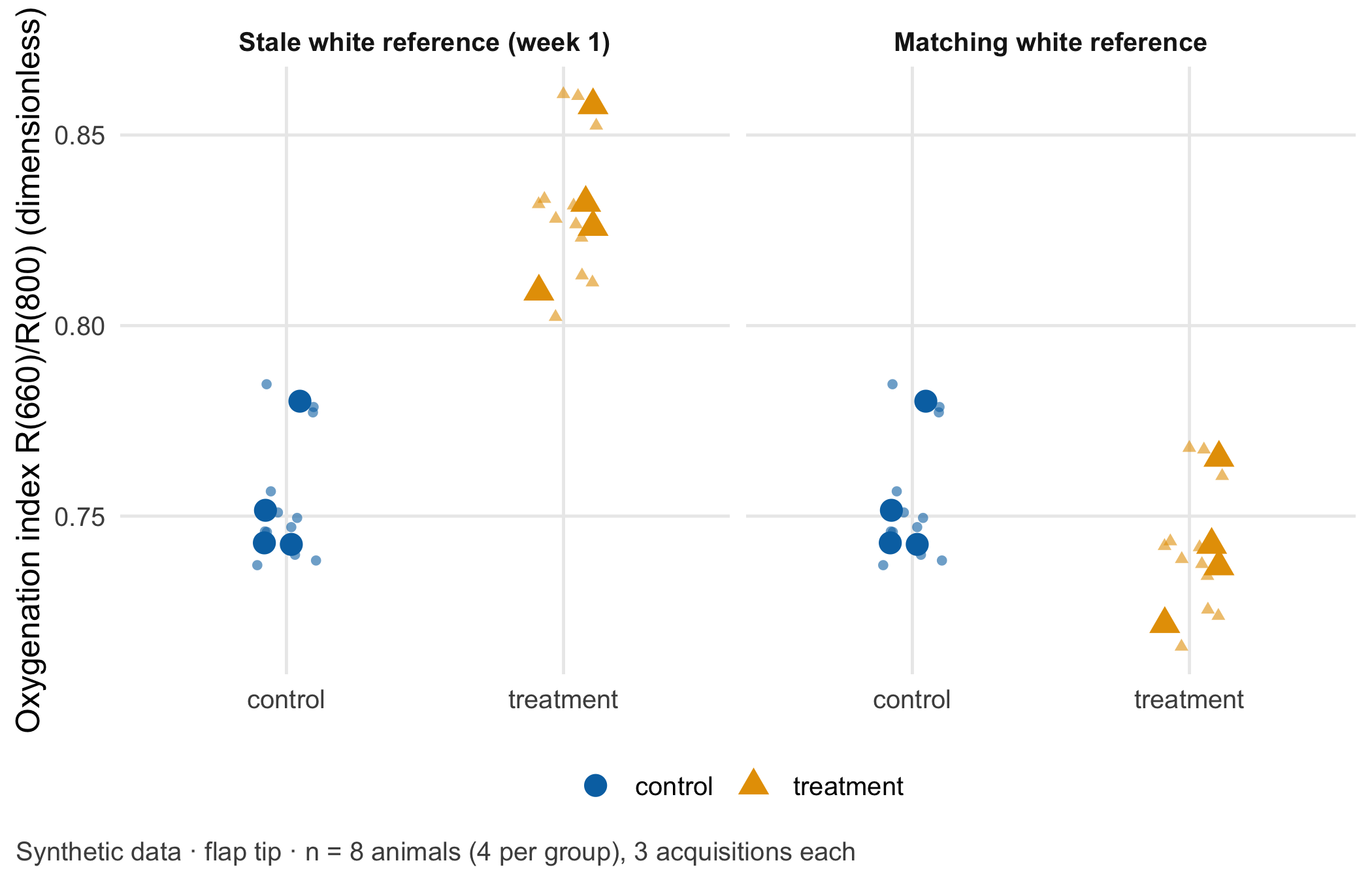
Two lessons sit in this table. With the stale white reference, the “effect” survives even the correct animal-level test (p = 0.0013 with 4 vs 4 animals): the right denominator does not protect against confounding. With the matching reference the mean index of the treated animals is 0.013 index units lower than that of the controls, and the animal-level test gives p = 0.35. The pixel-level test still reports p = 3.5e-12 for this chance difference, because it treats 600 tip pixels from eight animals as 600 independent observations. Figure 10.2 shows both levels.
Code
acq_tip <- spectra[spectra$region =="tip", ]animal_tip <-aggregate(index ~ animal + group + calibration, data = acq_tip, FUN = mean)facet_names <-c(stale ="Stale white reference (week 1)", matching ="Matching white reference")acq_tip$calibration <-factor(facet_names[acq_tip$calibration], levels = facet_names)animal_tip$calibration <-factor(facet_names[animal_tip$calibration], levels = facet_names)ggplot(acq_tip, aes(group, index, colour = group, shape = group)) +geom_point(position =position_jitter(width =0.12, height =0, seed =1), size =1.4, alpha =0.6) +geom_point(data = animal_tip, size =3.6, position =position_jitter(width =0.12, height =0, seed =2)) +facet_wrap(~ calibration) +scale_colour_manual(values =unname(cdsr_colours[c("blue", "orange")])) +scale_shape_manual(values = cdsr_shapes[1:2]) +labs(x =NULL, y ="Oxygenation index R(660)/R(800) (dimensionless)", colour =NULL, shape =NULL,caption ="Synthetic data · flap tip · n = 8 animals (4 per group), 3 acquisitions each") +theme_cdsr()
Figure 10.2: Oxygenation index R(660)/R(800) of the flap tip, dimensionless. Small symbols: region means per acquisition (three per animal); large symbols: animal means. Left: week-2 images calibrated with the stale week-1 white reference; right: with the matching reference. Synthetic data; independent unit: animal (n = 8, four per group).
Step 5 – index against a learning model on new animals. Before a learning model earns a place in the chain, it has to beat the simple index on animals it has never seen. We develop both methods on the four week-1 animals and test them on the four week-2 animals. The model is a k-nearest-neighbour classifier (k = 3) on the first three principal components of the full region-mean spectra; the principal components are computed from the training animals only. The task is to tell flap base from flap tip.
library(class)bands <-paste0("nm", wl)train <- spectra[spectra$week ==1& spectra$calibration =="matching", ]# Index baseline: threshold halfway between the mean index of base and tip in the training animalsthreshold <-mean(tapply(train$index, train$region, mean))# Learning model: principal components from training spectra only, then k-nearest neighbourspca <-prcomp(train[, bands], center =TRUE)evaluate <-function(cal) { test <- spectra[spectra$week ==2& spectra$calibration == cal, ] pred_index <-ifelse(test$index > threshold, "base", "tip") scores_test <-predict(pca, test[, bands])[, 1:3] pred_model <-as.character(knn(pca$x[, 1:3], scores_test, cl = train$region, k =3))data.frame(calibration = cal, test_animals =length(unique(test$animal)), test_spectra =nrow(test),accuracy_index =mean(pred_index == test$region), accuracy_model =mean(pred_model == test$region))}comparison <-rbind(evaluate("matching"), evaluate("stale"))stopifnot(length(intersect(unique(train$animal), unique(spectra$animal[spectra$week ==2]))) ==0)comparison
stopifnot(comparison$accuracy_index[1] >= comparison$accuracy_model[1], # the model does not beat the index comparison$accuracy_index[2] ==0.5, comparison$accuracy_model[2] ==0.5)
With the matching calibration, the index classifies 100% of the 24 test spectra correctly and the model 92%. The more flexible model brings no gain here, so the index remains the reference method in the model passport (Chapter 27). With the stale calibration both drop to 50%: every flap tip now looks like a flap base. A learning model does not repair an illumination error; it learns on top of it. The independent test denominator is four animals, not 24 spectra.
NoteOther implementation: Python with scikit-image and PyTorch
Hyperspectral pipelines are often written in Python. scikit-image (version 0.26.0 in November 2026) provides tested image operators such as filtering, registration and region measurements; most of them accept a channel_axis argument, and for a cube stored as rows × columns × bands this must be set to the spectral axis, otherwise the filter mixes neighbouring wavelengths (Walt et al. 2014). PyTorch connects to pretrained networks (Paszke et al. 2019). Networks with ImageNet weights, as in the transfer learning tutorial, expect three colour channels normalised with ImageNet means; a 101-band cube needs a new first layer, whose weights then cannot be transferred. Pretrained hyperspectral weights from research code are only usable if wavelength grid, calibration (reflectance, not raw counts), spatial resolution and band order match. For a fair comparison with this lab, both implementations must receive the identical calibrated reflectance table, the same animal-wise split (week-1 animals for development, week-2 animals for testing), the same index definition and the same accuracy computed per spectrum and per animal. Status: conceptual comparison, not run.
10.4 Counter-check
Predict first, then compute. Suppose the replacement lamp had been only brighter, with exactly the same spectral shape as the original. Would the stale white reference still inflate the index? And would the grey check tile still fail?
The ratio index survives a pure change in brightness: it stays within a few per cent of the true value, and the grey tile’s index stays within tolerance. The grey tile’s mean reflectance, however, rises to about 0.60 instead of 0.50, so the check still flags a problem with absolute reflectance. A change in the lamp’s colour affects the index; a change in brightness affects absolute values. The grey tile should be read on both quantities.
WarningCommon mistake
“A ratio index needs no calibration.” A ratio cancels everything that scales all wavelengths alike, such as distance, exposure time or a brighter lamp of the same colour. It does not cancel anything that changes the spectral shape: a new lamp type, an ageing bulb, daylight from a window or a different filter. A white reference recorded under the actual light remains necessary.
A design counter-check needs no code: if animals of both groups had been imaged in alternating order in both weeks, as ARRIVE item 4b recommends for the order of measurements (Percie du Sert et al. 2020), the lamp change would have shifted both groups alike and could not have produced a group difference.
10.5 Consequences for patients and operations
Wrong tissue interpretation. The same artefact in a clinical setting would make poorly oxygenated tissue look better oxygenated than it is. A surgeon judging a flap by such a value might delay a revision. The measurement assumption that protects against this is checkable: a grey reference tile imaged at every session has an index of 1.00 ± 0.02 and a mean reflectance of 0.50 ± 0.01. The failure mode is equally concrete: a lamp change without a new white reference shifts every index of that session by the same factor.
Animals and the 3Rs. A false positive treatment effect in an animal study has consequences beyond the abstract. It invites follow-up experiments, and therefore more animals, to pursue an effect that was never there. Reduction in the sense of the 3Rs starts with analyses that use the animal as the unit and designs that avoid confounding (NC3Rs 2026). Reporting the experimental unit and the order of measurements is part of ARRIVE (Percie du Sert et al. 2020).
Regulation. In this preclinical study the camera is a research instrument. If the same index were offered to clinicians to assess flap perfusion, its intended purpose would decide whether the software is a medical device and which class applies; Chapter 22 works through such an intended purpose.
Data protection and security. Animal data are not personal data. In a human study, wound and skin images can show tattoos, faces or rare findings and become identifiable; Chapter 23 covers this. The white reference and calibration files are part of the measurement. Storing them with a version and a checksum, so that the analysis can prove which file it used, is an integrity control of the kind discussed in Chapter 24.
10.6 Look up and transfer
Reviewer question: The manuscript reports p < 0.001 for a difference in an oxygenation index between two groups of animals. What was the experimental unit, were both groups imaged in the same sessions, and which reference target shows that the calibration was stable across sessions?
Self-test: A follow-up study images six animals per group, with four acquisitions per animal and 50 pixels per region of interest. A colleague proposes to divide every spectrum by its own mean, “to remove the lamp”. How many independent units does the group comparison have, does the proposal remove a change in lamp colour, and which design change prevents the confounding in this chapter?
TipAnswer
The group comparison has 12 independent units, six animals per group; the 2,400 pixels per region and the 48 acquisitions are repeated measurements within animals. Dividing by the mean removes a change in brightness but not a change in spectral shape, so a lamp with a different colour still distorts the ratio \(R(660)/R(800)\); only a white reference recorded under the same lamp corrects it. Imaging animals of both groups in alternating or randomised order within every session prevents the lamp from coinciding with the group, and a grey reference tile at every session detects a calibration problem before any animal is analysed.
Annotated sources:
Lu and Fei (2014) introduces the hypercube, calibration and medical applications of hyperspectral imaging.
Holmer et al. (2018) describes how real perfusion parameters are computed from spectra and why the chapter’s index is only a simplification.
Lazic (2010) explains pseudoreplication with examples and is the basis for testing per animal.
Percie du Sert et al. (2020) (items 1b and 4b) asks for the experimental unit and the order of measurements to be reported.
NC3Rs (2026) frames the consequence of a false positive result for further animal use.
Walt et al. (2014) and Paszke et al. (2019) document the Python implementations named in the box.
10.7 Further reading
Chapter 19 – what happens when images of known animals end up in the test set.
Chapter 16 – how much uncertainty remains with four animals per group.
Chapter 27 – the model passport, where the index belongs as the reference method.
Holmer, Amadeus, Jörg Marotz, Philip Wahl, Michael Dau, and Peer W. Kämmerer. 2018. “Hyperspectral Imaging in Perfusion and Wound Diagnostics – Methods and Algorithms for the Determination of Tissue Parameters.”Biomedical Engineering / Biomedizinische Technik 63 (5): 547–56. https://doi.org/10.1515/bmt-2017-0155.
Lazic, Stanley E. 2010. “The Problem of Pseudoreplication in Neuroscientific Studies: Is It Affecting Your Analysis?”BMC Neuroscience 11: 5. https://doi.org/10.1186/1471-2202-11-5.
Percie du Sert, Nathalie, Viki Hurst, Amrita Ahluwalia, et al. 2020. “The ARRIVE Guidelines 2.0: Updated Guidelines for Reporting Animal Research.”PLOS Biology 18 (7): e3000410. https://doi.org/10.1371/journal.pbio.3000410.
Walt, Stéfan van der, Johannes L. Schönberger, Juan Nunez-Iglesias, et al. 2014. “Scikit-Image: Image Processing in Python.”PeerJ 2: e453. https://doi.org/10.7717/peerj.453.