17 Forecasting patient flow
R. Heller · Date: 2025-07-13 · Last changed: 2026-11-09
17.1 Case and decision
On Thursday afternoon the nurse manager of a fictitious emergency department plans the roster for the coming week. A dashboard shows the expected number of arrivals for every hour, with a band labelled “90% interval”. The manager has one standby nurse to place. The tempting rule is to staff each shift to the upper edge of the band and to put the standby nurse where the band is widest. Before following that rule, the manager asks the analyst a plain question: if the band says 90%, did it in fact contain the arrivals in nine out of ten hours in past weeks, and in which shifts did it fail? The answer decides where the standby nurse goes. If the band is too narrow in weekend late shifts, the cost of the error falls on patients who wait longer and on a late-shift team that is already stretched.
17.2 Core reading
Two different questions. A forecast and a simulation are often shown on the same planning screen, but they answer different questions (Table 17.1). A forecast says how many patients are likely to arrive if the process continues as before. It can be checked: wait a week and compare. A simulated capacity change, the topic of Chapter 18, says what would happen to waiting times if the department changed something, given an assumed stream of arrivals. It cannot be checked against data before the change is made; it is checked by verification and plausibility instead. A forecast is often the input of such a simulation, which is one more reason to know how good it is.
| Forecast (this chapter) | Simulated capacity change (Chapter 18) | |
|---|---|---|
| Question | How many arrivals next week, if the process continues? | What happens to waiting if we add or remove a resource? |
| Changes the system? | No | Yes, hypothetically |
| How it is checked | Against later data (backtest, then prospectively) | Verification of the model logic, plausibility against external figures |
| Typical failure | Interval too narrow, process changed | Wrong assumptions about service times or priorities |
The data and the honest benchmark. The lab generates 26 weeks of hourly arrivals at a fictitious department with about 92 arrivals per day. The series has a daily rhythm (quiet nights, busy late mornings), a weekly rhythm (busier Mondays), a change of season from week 15 (15% more arrivals, for example from leisure injuries) and one unusual surge: in week 21, arrivals double on the afternoons and evenings of Friday to Sunday. Every number is synthetic. Any forecasting method has to beat a simple reference that a planner could compute by hand: the arrivals in the same hour of the previous week. This seasonal naive forecast (Hyndman and Athanasopoulos 2021) already contains the daily and weekly rhythm. A more elaborate model that does not beat it in later weeks adds complexity without benefit.
Testing in later windows only. A forecast for next week may use only data that existed before next week. The lab therefore uses a rolling-origin backtest (Tashman 2000): the forecast origin moves forward one week at a time, from week 9 to week 26, and each time the next 168 hours are forecast from the data before the origin. This gives 18 forecast weeks with 3,024 forecast hours. The independent denominator is closer to 18 than to 3,024, because all hours of one forecast week share the same origin and the same conditions. The general method is described in Methods in R: Rolling-Origin Cross-Validation.
Two forecasts, two intervals. The reference forecast uses last week’s value with a normal-approximation interval from the forecast package (Hyndman and Khandakar 2008). The second forecast uses the mean of the same hour over the last four weeks with an interval taken from a Poisson distribution, an assumption that is common for counts. A 90% interval should contain the observed arrivals in about 90% of hours (calibration, here measured as coverage) and should be as narrow as possible given that (sharpness) (Gneiting et al. 2007).
| Method | MAE | Coverage | Early | Late | Night | Mean width | Cost per week |
|---|---|---|---|---|---|---|---|
| Same hour last week | 2.85 | 0.88 | 0.83 | 0.82 | 0.99 | 9.3 | 302 |
| Four-week mean, Poisson interval | 2.28 | 0.82 | 0.79 | 0.76 | 0.91 | 5.9 | 245 |
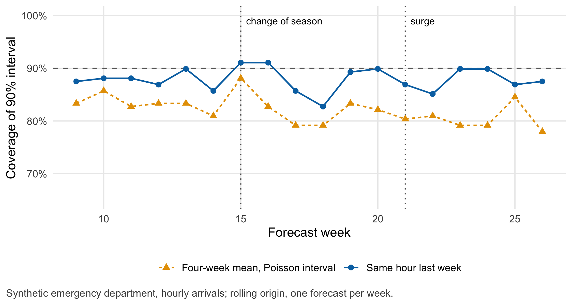
What the backtest shows. The four-week mean has the smaller point error (MAE 2.28 versus 2.85 arrivals per hour), but its Poisson interval contains the arrivals in only 82.0% of hours, and in the late shift in only 76.4%. The arrivals vary more than a Poisson model assumes. The reference interval reaches 87.9% overall, which looks close to 90%, but the average hides a split: 99.1% at night, where the band is needlessly wide, and 81.6% in the late shift, where it is too narrow. Point accuracy and interval calibration are separate properties, and calibration has to be checked where the decision is taken, here per shift. In the four weeks after the change of season both forecasts under-estimate arrivals, the four-week mean more so (by 0.48 versus 0.26 arrivals per hour on average), because most of its reference weeks still come from the old level. During the surge both intervals fail in the weekend late shifts.
The most important assumption. A forecast interval describes uncertainty under the assumption that next week’s arrivals come from the same process as the training weeks. It says nothing about events of a kind that the training window did not contain. The surge in week 21 is such an event. No interval built from past weeks could have anticipated it; that needs a separate signal, for example an event calendar or a heat warning, and a rule for what the department does when the signal fires.
Errors do not cost the same at every hour. One patient more than planned at 3 a.m., with a thin night team, has other consequences than one patient more at 11 a.m. The lab therefore weights errors by shift. The weights are an assumption that the department has to agree on; with other weights the ranking of the two methods can change. The point of writing them down is that the choice of method becomes a discussable decision instead of a by-product of a software default.
Question for the workshop: Your group plans the standby nurse for next week from Table 17.2. Which shift would you protect, which interval would you use, and what would you tell the late-shift team about the 90% label?
17.3 Lab
The lab follows the order of a real backtest: generate (or import) the series, fix the forecast origins, forecast only from data before each origin, and evaluate per week and per shift.
NoteR start command
From the root of the book repository, render the chapter (this runs all code, including the figures of the core reading):
quarto render chapters/b17-forecasting-patient-flow.qmd --to htmlTo run only the Lab code in a fresh R session, start from the chapters/ folder:
Rscript -e 'source(knitr::purl("b17-forecasting-patient-flow.qmd", output = tempfile(fileext = ".R"), quiet = TRUE))'The chapter writes the synthetic hourly series to data/b17-ed-arrivals.csv.
17.3.1 The synthetic arrival series
Arrivals per hour are drawn from a negative binomial distribution around an expected value that combines a daily profile, a weekly profile, the change of season and the surge. A day-level factor adds variation between days. The negative binomial allows more variation than a Poisson distribution, which is what real arrival counts often show.
set.seed(1717)
n_weeks <- 26
hours <- expand.grid(hour = 0:23, day = 1:7, week = 1:n_weeks)   # day 1 = Monday
hours <- hours[order(hours$week, hours$day, hours$hour), ]
hours$t <- seq_len(nrow(hours))                                    # running hour index

simulate_arrivals <- function(hours, day_shape = 80, nb_size = 6) {
  # expected arrivals per hour of the day (0-23 h): quiet night, busy late morning
  daily_profile <- c(1.6, 1.3, 1.1, 1.0, 1.0, 1.2, 1.8, 2.8, 4.0, 5.0, 5.6, 5.8,
                     5.6, 5.4, 5.2, 5.0, 5.0, 5.1, 5.0, 4.6, 4.0, 3.3, 2.6, 2.0)
  weekly <- c(1.12, 1.02, 1.00, 0.98, 1.00, 0.96, 0.94)             # Monday to Sunday
  season <- ifelse(hours$week >= 15, 1.15, 1.00)                     # change of season
  surge <- ifelse(hours$week == 21 & hours$day %in% 5:7 & hours$hour >= 14, 2.0, 1.0)
  day_key <- paste(hours$week, hours$day)
  day_factor <- if (is.finite(day_shape)) rgamma(length(unique(day_key)), day_shape, day_shape) else
    rep(1, length(unique(day_key)))                                  # day-to-day variation
  names(day_factor) <- unique(day_key)
  mu <- daily_profile[hours$hour + 1] * weekly[hours$day] * season * surge * day_factor[day_key]
  if (is.finite(nb_size)) rnbinom(nrow(hours), size = nb_size, mu = mu) else rpois(nrow(hours), mu)
}
hours$arrivals <- simulate_arrivals(hours)

# shifts: early 06-14, late 14-22, night 22-06 (a night shift belongs to the day on which it starts)
hours$shift <- ifelse(hours$hour >= 6 & hours$hour < 14, "early",
                      ifelse(hours$hour >= 14 & hours$hour < 22, "late", "night"))
hours$shift_day <- ifelse(hours$hour < 6, (hours$day - 2) %% 7 + 1, hours$day)

b17_daily <- tapply(hours$arrivals, paste(hours$week, hours$day), sum)
b17_daily_mean <- mean(b17_daily)
stopifnot(nrow(hours) == 26 * 168, all(hours$arrivals >= 0), !anyNA(hours$arrivals))
head(hours[, c("week", "day", "hour", "shift", "arrivals")], 3)
#> week day hour shift arrivals
#> 1 1 1 0 night 3
#> 2 1 1 1 night 0
#> 3 1 1 2 night 0summary(as.numeric(b17_daily))#> Min. 1st Qu. Median Mean 3rd Qu. Max.
#> 52.00 78.00 90.00 91.78 106.75 169.00if (dir.exists("../data")) {
write.csv(hours[, c("week", "day", "hour", "shift", "arrivals")], "../data/b17-ed-arrivals.csv", row.names = FALSE)
}17.3.2 Rolling-origin backtest
The function below loops over the forecast origins. The stopifnot() lines are the heart of the lab: every training hour lies before every test hour, and the seasonal naive forecast from the forecast package equals the hand computation “same hour last week”.
library(forecast)
backtest <- function(y, origin_weeks = 9:26, m = 168, level = 0.90) {
  out <- vector("list", length(origin_weeks))
  for (i in seq_along(origin_weeks)) {
    w <- origin_weeks[i]
    train_idx <- seq_len((w - 1) * m)                 # all hours before the origin
    test_idx <- (w - 1) * m + seq_len(m)              # the 168 hours after the origin
    stopifnot(max(train_idx) < min(test_idx))         # no information from the future
    y_train <- y[train_idx]
    # reference: seasonal naive (same hour last week), normal-approximation interval
    fc <- snaive(ts(y_train, frequency = m), h = m, level = 100 * level)
    point_sn <- as.numeric(fc$mean)
    stopifnot(isTRUE(all.equal(point_sn, y_train[length(y_train) - m + seq_len(m)])))
    # alternative: mean of the same hour in the last four weeks, Poisson interval
    lambda <- rowMeans(matrix(tail(y_train, 4 * m), nrow = m))
    out[[i]] <- rbind(
      data.frame(method = "Same hour last week", week = w, t = test_idx, y = y[test_idx],
                 point = point_sn, lo = pmax(0, as.numeric(fc$lower)), hi = as.numeric(fc$upper)),
      data.frame(method = "Four-week mean, Poisson interval", week = w, t = test_idx, y = y[test_idx],
                 point = lambda, lo = qpois((1 - level) / 2, lambda), hi = qpois(1 - (1 - level) / 2, lambda))
    )
  }
  do.call(rbind, out)
}
bt <- backtest(hours$arrivals)
bt <- merge(bt, hours[, c("t", "day", "hour", "shift", "shift_day")], by = "t")
bt$covered <- bt$y >= bt$lo & bt$y <= bt$hi       # inside the 90% interval?
bt$abs_err <- abs(bt$y - bt$point)
stopifnot(length(unique(bt$week)) == 18, nrow(bt) == 2 * 18 * 168)
17.3.3 Evaluation per method, week and shift
Planned capacity is taken to be the upper edge of the interval. A patient above that edge counts as an excess patient; an unused planned place counts as idle capacity. The weights are an assumption for teaching: an excess patient costs 1 point in the early shift, 2 in the late shift and 3 at night; an idle place costs 0.25 points.
w_excess <- c(early = 1, late = 2, night = 3)               # cost points per excess patient (assumption)
w_idle <- 0.25                                              # cost points per idle planned place (assumption)
bt$excess <- pmax(0, bt$y - bt$hi)
bt$idle <- pmax(0, bt$hi - bt$y)
bt$cost <- w_excess[bt$shift] * bt$excess + w_idle * bt$idle

key <- c("Same hour last week" = "snaive", "Four-week mean, Poisson interval" = "mean4")
b17_mae <- tapply(bt$abs_err, key[bt$method], mean)
b17_cov <- tapply(bt$covered, key[bt$method], mean)
b17_cov_shift <- tapply(bt$covered, list(key[bt$method], bt$shift), mean)
b17_width <- tapply(bt$hi - bt$lo, key[bt$method], mean)
b17_cost_week <- tapply(bt$cost, key[bt$method], sum) / 18
b17_summary <- data.frame(
  method = names(key), mae = b17_mae[key], coverage = b17_cov[key],
  early = b17_cov_shift[key, "early"], late = b17_cov_shift[key, "late"], night = b17_cov_shift[key, "night"],
  width = b17_width[key], cost_week = b17_cost_week[key]
)
b17_summary
#> method mae coverage early late
#> snaive Same hour last week 2.852183 0.8789683 0.8293651 0.8164683
#> mean4 Four-week mean, Poisson interval 2.276124 0.8201058 0.7886905 0.7638889
#> night width cost_week
#> snaive 0.9910714 9.281171 301.6320
#> mean4 0.9077381 5.938161 244.9722# statements made in the core reading
# mean error (forecast minus observed) in the four weeks after the change of season
b17_bias_season <- tapply((bt$point - bt$y)[bt$week %in% 15:18], key[bt$method][bt$week %in% 15:18], mean)
# coverage in the late shifts of the surge weekend (week 21, Friday to Sunday)
in_surge <- bt$week == 21 & bt$day %in% 5:7 & bt$shift == "late"
b17_surge_cov <- tapply(bt$covered[in_surge], key[bt$method][in_surge], mean)
round(b17_bias_season, 2); round(b17_surge_cov, 2)#> mean4 snaive
#> -0.48 -0.26#> mean4 snaive
#> 0.38 0.67# statements made in the core reading
stopifnot(b17_mae["mean4"] < b17_mae["snaive"], # smaller point error
b17_cov["mean4"] < 0.85, # Poisson interval too narrow
b17_cov_shift["snaive", "night"] > 0.95, # reference too wide at night ...
b17_cov_shift["snaive", "late"] < 0.85, # ... and too narrow in the late shift
b17_bias_season["mean4"] < b17_bias_season["snaive"], # larger under-forecast after the season change
b17_bias_season["snaive"] < 0,
all(b17_surge_cov < 0.7)) # both intervals fail in the surge late shiftsThe point forecasts of the two methods differ in a way that is easy to see in a single week. Figure 17.2 shows the surge weekend of week 21: in its late shifts the observed arrivals stay inside the band in only 38% (four-week mean) and 67% (reference) of hours.
library(ggplot2)
surge <- bt[bt$week == 21 & bt$day %in% 5:7, ]
surge$hour_since_fri <- (surge$day - 5) * 24 + surge$hour
ggplot(surge, aes(hour_since_fri)) +
  geom_ribbon(aes(ymin = lo, ymax = hi), fill = "grey80") +
  geom_line(aes(y = point), linewidth = 0.5) +
  geom_point(aes(y = y), size = 1.3) +
  facet_wrap(~ method, ncol = 1) +
  scale_x_continuous(breaks = seq(0, 72, by = 12)) +
  labs(x = "Hour since Friday 00:00 (week 21)", y = "Arrivals per hour",
       caption = "Grey band: 90% interval; line: point forecast; points: observed arrivals.") +
  theme_cdsr()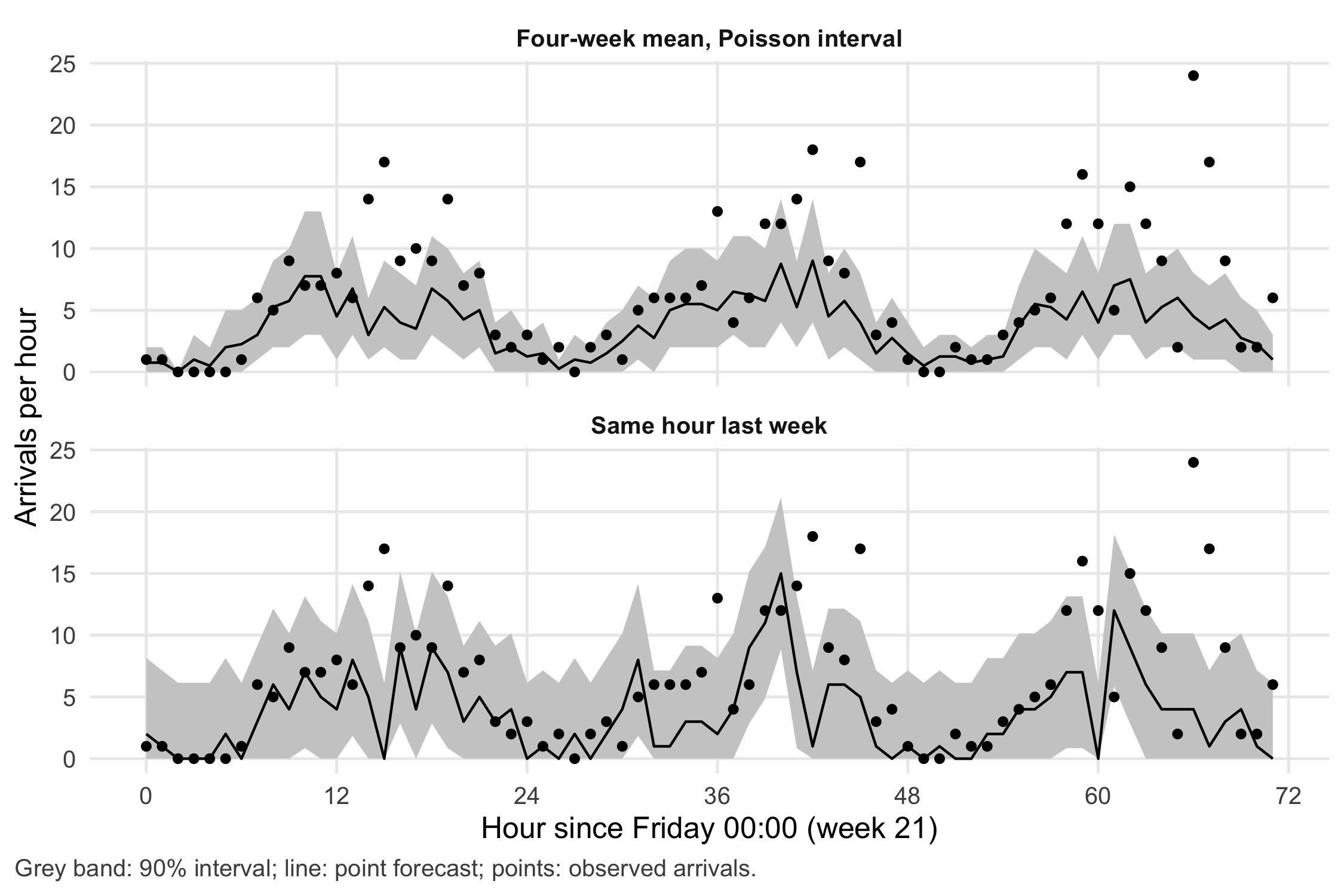
17.3.4 A shift map
The shift map turns the hourly results into the unit of the decision. Each cell shows the coverage of the 90% interval for one weekday and shift, pooled over the 18 forecast weeks.
shiftmap <- aggregate(covered ~ method + shift_day + shift, data = bt, FUN = mean)
shiftmap$weekday <- factor(c("Mon", "Tue", "Wed", "Thu", "Fri", "Sat", "Sun")[shiftmap$shift_day],
                           levels = c("Mon", "Tue", "Wed", "Thu", "Fri", "Sat", "Sun"))
shiftmap$shift <- factor(shiftmap$shift, levels = c("night", "late", "early"))
ggplot(shiftmap, aes(weekday, shift, fill = covered)) +
  geom_tile(colour = "white") +
  geom_text(aes(label = scales::percent(covered, accuracy = 1),
                colour = covered < 0.8), size = 3, show.legend = FALSE) +
  scale_fill_gradient(low = "grey20", high = "grey95", limits = c(0.5, 1), breaks = c(0.5, 0.75, 1),
                      labels = scales::label_percent(), name = "Coverage") +
  scale_colour_manual(values = c(`TRUE` = "white", `FALSE` = "black")) +
  facet_wrap(~ method, ncol = 2) +
  labs(x = NULL, y = NULL, caption = "Nominal coverage 90%. Night shift is assigned to the day on which it starts.") +
  theme_cdsr() +
  theme(panel.grid = element_blank(), legend.key.width = grid::unit(1.5, "cm"))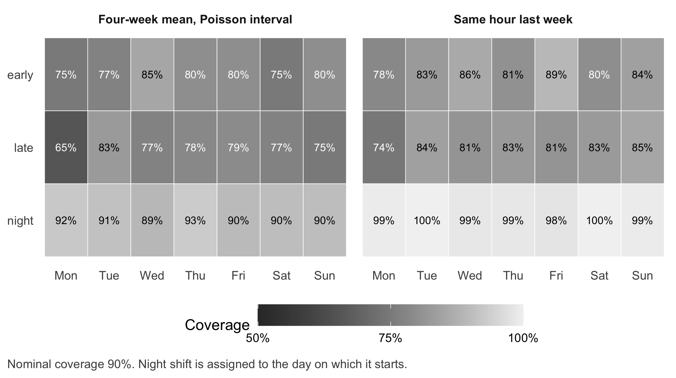
b17_worst <- shiftmap[order(shiftmap$covered), ][1:3, c("method", "weekday", "shift", "covered")]
b17_worst
#> method weekday shift covered
#> 15 Four-week mean, Poisson interval Mon late 0.6527778
#> 16 Same hour last week Mon late 0.7430556
#> 1 Four-week mean, Poisson interval Mon early 0.7500000stopifnot(b17_worst$weekday[1] == b17_worst$weekday[2], b17_worst$shift[1] == "late",
b17_worst$shift[2] == "late", b17_worst$method[1] != b17_worst$method[2])The lowest cell for both methods is the Monday late shift (65% and 74%), the busiest shift of the week, where the extra variation of the counts matters most. For the manager in the case, this is the actionable result: the label “90%” is not a property of the dashboard but of each shift, and it holds neither for the late shifts nor (in the other direction) for the nights.
17.3.5 Weighted error cost
b17_cost_shift <- aggregate(cost ~ method + shift, data = bt, FUN = function(x) sum(x) / 18)
b17_cost_shift
#> method shift cost
#> 1 Four-week mean, Poisson interval early 79.43056
#> 2 Same hour last week early 100.61438
#> 3 Four-week mean, Poisson interval late 113.19444
#> 4 Same hour last week late 115.94460
#> 5 Four-week mean, Poisson interval night 52.34722
#> 6 Same hour last week night 85.07299stopifnot(all(b17_cost_shift$cost >= 0))With these weights the four-week mean has the lower weekly cost (245 versus 302 points), because the wide reference band leaves many more planned places idle; about half of these additional idle places fall in night shifts. Raise the weight of an excess night patient or of an excess late-shift patient, and the comparison moves towards the wider band. The weights encode a value judgement about who carries which error, which belongs in the roster discussion, not in the code alone.
17.4 Counter-check
Change one assumption about the process: suppose arrivals were truly Poisson, without extra variation between days or hours. Predict before running: will the coverage of the Poisson interval move towards 90%? Will the reference interval still be too wide at night and too narrow in the late shift?
set.seed(1718)
y_poisson <- simulate_arrivals(hours, day_shape = Inf, nb_size = Inf)   # same rhythm, no overdispersion
bt_p <- backtest(y_poisson)
bt_p <- merge(bt_p, hours[, c("t", "shift")], by = "t")
bt_p$covered <- bt_p$y >= bt_p$lo & bt_p$y <= bt_p$hi
b17_cov_p <- tapply(bt_p$covered, list(key[bt_p$method], bt_p$shift), mean)
round(cbind(overall = tapply(bt_p$covered, key[bt_p$method], mean), b17_cov_p), 3)
#> overall early late night
#> mean4 0.907 0.900 0.885 0.937
#> snaive 0.884 0.852 0.816 0.982stopifnot(mean(bt_p$covered[key[bt_p$method] == "mean4"]) > b17_cov["mean4"],
b17_cov_p["snaive", "night"] > b17_cov_p["snaive", "late"])Under the Poisson assumption the Poisson interval covers 90.7% of hours, close to its nominal level. The reference interval still covers 98.2% at night and 81.6% in the late shift: its width is the same for every hour, while the variation of counts grows with the expected number. The counter-check separates two reasons for poor coverage. One is a wrong distributional assumption (Poisson for overdispersed counts); the other is an interval that ignores how uncertainty changes over the day. Both are properties of the method, not of the hospital.
17.5 Consequences for patients and operations
Ethics and distribution of burden. A forecast used for rostering shifts errors onto concrete people. If intervals are systematically too narrow in weekend late shifts, the patients arriving then wait longer and the late-shift team absorbs the overload, often the same staff week after week. Reporting coverage per shift, not only overall, makes this distribution visible. The cost weights in the lab are a place to make the value judgement explicit and to involve the nursing team, not only the analyst.
Regulation. Indirect. A forecast of arrival counts for staffing has no diagnostic or therapeutic purpose for an individual patient; whether such software falls under medical device rules is a question of its intended purpose (Chapter 22). The question would change if the same model were used to prioritise individual patients: the AI Act lists “emergency healthcare patient triage systems” among high-risk uses in Annex III, point 5(d) (European Parliament and Council of the European Union 2024). As of November 2026.
Data protection. The model needs counts per hour, not patient records. Aggregating timestamps to hourly counts before analysis is a direct application of data minimisation under Art. 5(1)(c) of the General Data Protection Regulation (European Parliament and Council of the European Union 2016). Very small counts in rare categories (for example arrivals by a specific transport mode at night) can still point to individuals when combined with local knowledge; Chapter 20 and Chapter 26 treat small aggregates.
Security and availability. If the forecast service fails, the department needs a fallback that works without it. The seasonal naive forecast is that fallback: last week’s arrivals, available from any routine report.
17.6 Look up and transfer
- Reviewer question: Which forecast origins and horizons were evaluated, was any information from after the origin used (for example smoothing over the whole series or a calendar compiled later), and what is the interval coverage per shift, with the number of forecast weeks as denominator?
- Self-test: A smaller department has on average 1.2 arrivals per hour at night, with many hours of zero arrivals. Its analyst compares two forecasts by the mean absolute percentage error (MAPE) over all hours and reports that model X is “40% better”. What is the problem with this metric here, and what would you report instead?
TipAnswer
Percentage errors divide by the observed value. In hours with zero arrivals they are undefined, and in hours with one arrival a single extra patient is an error of 100%, so the night hours dominate the comparison. Report the mean absolute error in arrivals per hour, or a scaled error that divides by the error of the seasonal naive reference (the MASE) (Hyndman and Koehler 2006), separately for each shift and with the number of forecast weeks. For the interval, report coverage per shift.
- Annotated sources:
- Hyndman and Athanasopoulos (2021) is the open textbook for benchmark methods, prediction intervals and time series cross-validation used here (simple methods, time series cross-validation).
- Hyndman and Khandakar (2008) documents the
forecastpackage and its automatic methods; the lab uses itssnaive(). - Jones et al. (2008) compared several forecasting methods for daily emergency department volumes at three hospitals and found that calendar-based regression was a reasonable approach, while more complex methods did not give consistently better post-sample accuracy.
- Tashman (2000) reviews out-of-sample evaluation and rolling forecast origins.
- Gneiting et al. (2007) define the goal “maximise sharpness subject to calibration” for probabilistic forecasts.
- Hyndman and Koehler (2006) discuss accuracy measures, including scaled errors for series with zeros.
In W6 (teaching unit 21) learners compare forecasts against “same hour last week” in later windows and hand in a table with horizon, error measure, interval coverage and one shift with possible harm. In W3 the chapter serves as a transfer case: the same distinction between ranking, calibration and decision cost appears for diagnostic models in Chapter 6.
17.7 Further reading
- Chapter 18 for the second question on the planning screen: what a capacity change would do, given arrivals.
- Chapter 6 for calibration and decision thresholds in a diagnostic setting.
- Chapter 20 for monitoring a deployed tool, including drift after a change of season or practice.
- Methods in R: Forecast Accuracy Metrics for the definitions of MAE, RMSE, MAPE and scaled errors.
- Methods in R: Seasonal Decomposition (STL) for separating daily, weekly and seasonal components.
- CTTIR Tutorials: Rolling-Origin Cross-Validation for a step-by-step tutorial on the backtest design.
- CTTIR Courses, Course 3, Week 2 Session 5: Time series basics for a hands-on introduction to time series in R.