15 Mechanistic models and pharmacometrics
R. Heller · Date: 2026-04-12 · Last changed: 2026-11-09
WarningVirtual parameters only
Every dose, volume and clearance in this chapter is a virtual model input for a fictitious compound. Nothing here is a dosing recommendation, and the numbers do not describe any real drug or patient group.
15.1 Case and decision
A doctoral researcher in clinical pharmacology is writing the sampling section of a protocol for a fictitious intravenous compound in injured adults. The ethics committee has asked the team to keep blood sampling to a minimum, and the trial unit can process two samples per person. The researcher must choose the two times. A senior colleague suggests taking both samples late, at 6 and 8 hours, “because by then the drug is evenly distributed”. Another proposes one sample shortly after the injection and one late. The protocol will fix the times for every participant, and they cannot be changed after the first person is enrolled. Which schedule allows the clearance and the volume of distribution to be estimated separately – and how precisely? The chapter answers with a one-compartment model and virtual parameters only.
15.2 Core reading
From mass balance to a concentration curve. A one-compartment model treats the body as one well-mixed volume. Let A(t) be the amount of compound in the body (mg) and C(t) the plasma concentration (mg/L). The volume of distribution V (L) links the two: C = A / V. It is a proportionality constant, not an anatomical space. The clearance CL (L/h) is the volume of plasma cleared of the compound per hour, so the elimination rate is CL × C, in L/h × mg/L = mg/h. The mass balance says that the amount in the body falls exactly by what is eliminated:
\[ \frac{dA}{dt} = -\,CL \cdot C = -\frac{CL}{V}\,A, \qquad A(0) = \text{dose}. \]
The units check: (L/h) / L × mg = mg/h. After a single intravenous bolus, the solution is C(t) = (dose / V) · exp(−(CL / V) · t). The ratio k = CL / V (1/h) is the elimination rate constant, the half-life is ln 2 · V / CL, and the area under the curve from zero to infinity is dose / CL (mg·h/L). With the virtual values dose = 100 mg, V = 20 L and CL = 5 L/h, the initial concentration is 5 mg/L, the half-life 2.77 h and the AUC 20 mg·h/L.
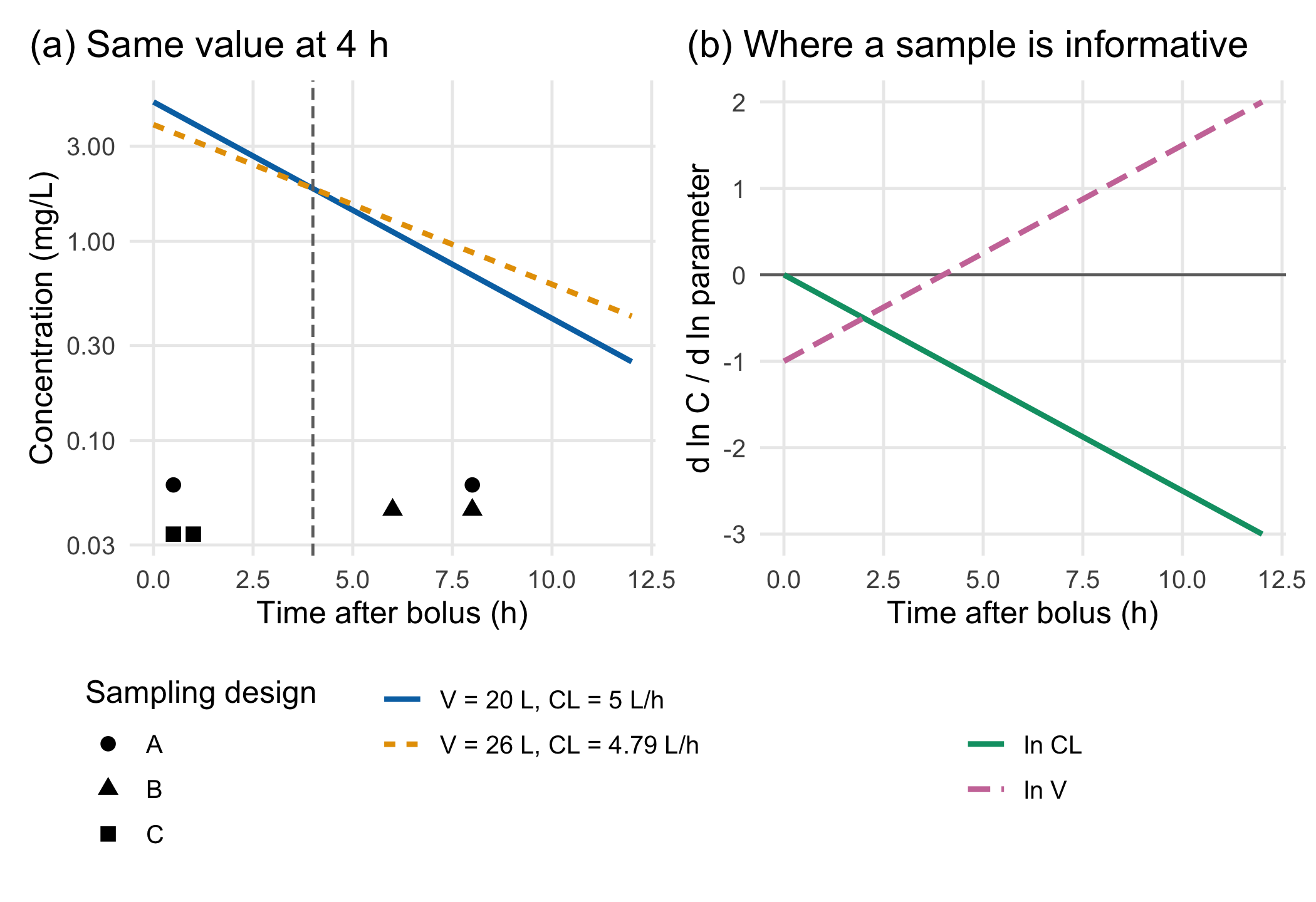
Two parameters, one sample. On a logarithmic scale the curve is a straight line: ln C(t) = ln(dose / V) − k · t. The intercept carries the volume, the slope carries the ratio CL / V. One sample, or two samples at the same time, gives one equation for two unknowns. Panel (a) of Figure 15.1 shows two virtual parameter sets that produce exactly the same concentration at 4 h: V = 20 L with CL = 5 L/h, and V = 26 L with CL = 4.79 L/h. A design that measures only at 4 h cannot tell them apart. This is structural non-identifiability (Bellman and Åström 1970): no amount of measurement precision helps.
Where a sample is informative. Panel (b) shows the normalised sensitivities: how much ln C changes when ln V or ln CL changes. For the volume, the sensitivity is −1 + k · t; it is zero at t = V / CL = 4 h. A sample taken then is blind to V, given CL. For the clearance, the sensitivity is −k · t; early samples hardly inform it. The two parameters are separated best when the samples sit at times where the two curves differ in shape, early and late.
Two samples, four designs. With a proportional measurement error of 10% (assumption), the expected standard errors follow from these sensitivities (the Fisher information, linearised at the virtual values). Table 15.1 compares four designs. The early-and-late design A estimates both parameters to within about 7–11%. Two late samples (design B) leave the volume uncertain by about 50%, because the intercept must be extrapolated back over six hours. Design B is structurally identifiable, yet practically the data hardly constrain V – the distinction between structural and practical identifiability (Raue et al. 2009). Two early samples (design C) estimate the volume reasonably but the clearance hardly at all. Two samples at the same time (design D) cannot separate the parameters at all. The simulated spread over 2,000 virtual repetitions agrees with the linearised values. Intuitively, a straight line through two points that are close together is poorly anchored: a 10% error at either point tilts the line, and the tilt is magnified when the line is extended back to time zero to read off the volume, or forward to infinity to obtain the area under the curve.
| Design | Sampling times (h) | V expected | V simulated | CL expected | CL simulated |
|---|---|---|---|---|---|
| A: early and late | 0.5 and 8 | 11 | 11 | 7 | 7 |
| B: both late | 6 and 8 | 50 | 50 | 22 | 21 |
| C: both early | 0.5 and 1 | 22 | 23 | 92 | 85 |
| D: same time twice | 4 and 4 | not identifiable | not identifiable | not identifiable | not identifiable |
The most important assumption. These standard errors hold only if the structural model is right and the parameters are near the values used to compute them. The best design depends on the very parameters it is meant to estimate; the counter-check shows what happens when the clearance is lower than expected. Model-based design is therefore local: it needs prior knowledge and should be checked across a plausible parameter range.
Checking the arithmetic before the biology. Most mechanistic models have no closed-form solution and are solved numerically. Before any parameter is estimated, the lab therefore checks that the numerical solver reproduces the analytical curve of this simple model within a tolerance fixed in advance. A closed mass balance – the amount in the body plus the amount eliminated always equals the dose – is necessary but does not prove that the solution is accurate.
A baseline without a model. With many samples per person, non-compartmental analysis (NCA) estimates the clearance without assuming a compartment model: the AUC is computed from the measured concentrations with the trapezoidal rule and extrapolated to infinity, and CL = dose / AUC. The lab uses it as the baseline for a virtual person with nine samples. With two samples per person, NCA is not available, and the model carries the inference.
Beyond one person. Real participants differ: the clearance and the volume vary between people (interindividual variability), and every measurement carries assay and handling error (residual variability). Population pharmacokinetic models estimate both at once and let different people be sampled at different times (Mould and Upton 2012, 2013). Automated searches over model structures, for example with genetic algorithms (Sale and Sherer 2015), are a further step. Neither repairs a design in which the data cannot separate the parameters.
Question for the workshop. The colleague’s argument for late samples was that “the drug is evenly distributed by then”. In a one-compartment model this is true from the start. Which feature of a real compound would make early samples misleading, and what would that change in the design?
15.3 Lab
The lab needs deSolve, ggplot2 and patchwork and runs in about two seconds.
15.3.1 Step 1: parameters with units
dose_mg <- 100           # virtual intravenous bolus (mg) – model input, not a dosing recommendation
V_l <- 20                # virtual volume of distribution (L)
CL_l_h <- 5              # virtual clearance (L/h)
k_per_h <- CL_l_h / V_l  # elimination rate constant (1/h)
sigma_log <- 0.1         # proportional measurement error, SD on the log scale (assumption)
conc_analytic <- function(t, dose = dose_mg, V = V_l, CL = CL_l_h) dose / V * exp(-CL / V * t)  # mg/L
c(C0_mg_l = dose_mg / V_l, half_life_h = log(2) * V_l / CL_l_h, AUC_mg_h_l = dose_mg / CL_l_h)
#> C0_mg_l half_life_h AUC_mg_h_l
#> 5.000000 2.772589 20.00000015.3.2 Step 2: the numerical solver against the analytical solution
The model is written as a mass balance with two states: the amount in the body (A) and the cumulative amount eliminated (E). Before running the solver, the tolerance is fixed: the largest relative deviation from the analytical solution at the output times must not exceed 10−4. This is a thousand times smaller than the assumed 10% measurement error and below the precision of three significant digits used for reporting, so solver error cannot change any conclusion.
library(deSolve)
pk_rhs <- function(t, state, parms) {
  with(as.list(c(state, parms)), {
    conc <- A / V                                  # mg/L
    list(c(A = -CL * conc,                         # mg/h leaving the body
           E = CL * conc))                         # mg/h arriving in the eliminated pool
  })
}
times <- seq(0, 24, by = 0.25)                     # output grid (h)
state0 <- c(A = dose_mg, E = 0)
parms <- c(CL = CL_l_h, V = V_l)
solve_with <- function(method, ...) ode(y = state0, times = times, func = pk_rhs, parms = parms, method = method, ...)
solutions <- list(
  `lsoda, rtol = atol = 1e-8` = solve_with("lsoda", rtol = 1e-8, atol = 1e-8),
  `lsoda, defaults (1e-6)` = solve_with("lsoda"),
  `rk4, fixed step 0.25 h` = solve_with("rk4"),
  `Euler, fixed step 0.25 h` = solve_with("euler"))
tolerance <- 1e-4
reference <- conc_analytic(times)
solver_check <- data.frame(
  solver = names(solutions),
  max_relative_error = sapply(solutions, function(s) max(abs(s[, "A"] / V_l - reference) / reference)),
  max_mass_balance_error_mg = sapply(solutions, function(s) max(abs(s[, "A"] + s[, "E"] - dose_mg))))
solver_check$passes <- solver_check$max_relative_error <= tolerance
rownames(solver_check) <- NULL
solver_check
#> solver max_relative_error max_mass_balance_error_mg passes
#> 1 lsoda, rtol = atol = 1e-8 4.464623e-10 8.526513e-14 TRUE
#> 2 lsoda, defaults (1e-6) 2.921983e-08 7.105427e-14 TRUE
#> 3 rk4, fixed step 0.25 h 8.037602e-07 4.263256e-14 TRUE
#> 4 Euler, fixed step 0.25 h 1.777395e-01 2.842171e-14 FALSEstopifnot(solver_check$passes[1:3], # adaptive and rk4 solutions within tolerance
!solver_check$passes[4], # the check detects the inadequate Euler step
all(solver_check$max_mass_balance_error_mg < 1e-8)) # mass is conserved by every methodAll four methods conserve mass, yet the Euler solution deviates by up to 17.8% from the analytical curve. A closed mass balance is necessary, not sufficient; only the comparison with an independent reference reveals the error. The adaptive solver lsoda (Soetaert et al. 2010; Petzold 1983) passes with both tolerance settings.
15.3.3 Step 3: structural identifiability at a single time
V_alt <- 26                                          # a second virtual volume (L)
CL_alt <- uniroot(function(cl) conc_analytic(4, V = V_alt, CL = cl) - conc_analytic(4),
                  interval = c(0.1, 20))$root        # clearance that gives the same C at 4 h
c(CL_alt_l_h = CL_alt, C4_set1 = conc_analytic(4), C4_set2 = conc_analytic(4, V = V_alt, CL = CL_alt),
  C05_set1 = conc_analytic(0.5), C05_set2 = conc_analytic(0.5, V = V_alt, CL = CL_alt))
#> CL_alt_l_h C4_set1 C4_set2 C05_set1 C05_set2
#> 4.794632 1.839397 1.839397 4.412485 3.507380stopifnot(abs(conc_analytic(4) - conc_analytic(4, V = V_alt, CL = CL_alt)) < 1e-8,
abs(conc_analytic(0.5) / conc_analytic(0.5, V = V_alt, CL = CL_alt) - 1) > 0.1) # an early sample separates them15.3.4 Step 4: expected precision of each design
For a log-normal error with standard deviation σ, the covariance of the estimates of (ln V, ln CL) is approximately σ² (SᵀS)⁻¹, where each row of S holds the sensitivities d ln C / d ln V = −1 + k·t and d ln C / d ln CL = −k·t at one sampling time. The diagonal gives the squared standard errors on the log scale, which are approximately relative standard errors. A design whose matrix S has rank below 2 is not identifiable.
sens_log <- function(t, V = V_l, CL = CL_l_h) cbind(lnV = -1 + CL / V * t, lnCL = -CL / V * t)
expected_se <- function(t, V = V_l, CL = CL_l_h, sigma = sigma_log) {
  S <- sens_log(t, V, CL)
  if (qr(S)$rank < 2) return(c(lnV = Inf, lnCL = Inf))  # structurally non-identifiable
  sqrt(diag(sigma^2 * solve(crossprod(S))))
}
designs <- data.frame(label = c("A", "B", "C", "D"), t1 = c(0.5, 6, 0.5, 4), t2 = c(8, 8, 1, 4),
                      description = c("early and late", "both late", "both early", "same time twice"))
# Simulation check: 2,000 virtual repetitions of one person per design, two log concentrations each
simulate_design <- function(t1, t2, n_sim = 2000, V = V_l, CL = CL_l_h) {
  if (t1 == t2) return(c(lnV = NA, lnCL = NA, share_invalid = NA))
  y1 <- log(conc_analytic(t1, V = V, CL = CL)) + rnorm(n_sim, 0, sigma_log)
  y2 <- log(conc_analytic(t2, V = V, CL = CL)) + rnorm(n_sim, 0, sigma_log)
  k_hat <- (y1 - y2) / (t2 - t1)                       # slope of the log-linear line
  V_hat <- dose_mg / exp(y1 + k_hat * t1)              # back-extrapolated intercept
  CL_hat <- k_hat * V_hat
  ok <- CL_hat > 0                                     # a negative slope gives no valid clearance
  c(lnV = sd(log(V_hat)), lnCL = sd(log(CL_hat[ok])), share_invalid = mean(!ok))
}
set.seed(15151)
expected <- t(mapply(function(a, b) expected_se(c(a, b)), designs$t1, designs$t2))
simulated <- t(mapply(simulate_design, designs$t1, designs$t2))
pct <- function(x) ifelse(is.finite(x), cdsr_number(100 * x, 0), "not identifiable")
design_table <- data.frame(
  Design = paste(designs$label, designs$description, sep = ": "),
  `Sampling times (h)` = paste(designs$t1, "and", designs$t2),
  `V expected` = pct(expected[, "lnV"]), `V simulated` = pct(simulated[, "lnV"]),
  `CL expected` = pct(expected[, "lnCL"]), `CL simulated` = pct(simulated[, "lnCL"]),
  check.names = FALSE)
design_table
#> Design Sampling times (h) V expected V simulated
#> 1 A: early and late 0.5 and 8 11 11
#> 2 B: both late 6 and 8 50 50
#> 3 C: both early 0.5 and 1 22 23
#> 4 D: same time twice 4 and 4 not identifiable not identifiable
#> CL expected CL simulated
#> 1 7 7
#> 2 22 21
#> 3 92 85
#> 4 not identifiable not identifiablestopifnot(
all(abs(simulated[1:2, c("lnV", "lnCL")] / expected[1:2, ] - 1) < 0.1), # linearisation confirmed (A, B)
abs(simulated[3, "lnV"] / expected[3, "lnV"] - 1) < 0.1, # and for V in design C
all(is.infinite(expected[4, ])), # design D is not identifiable
expected[1, "lnV"] < expected[2, "lnV"], expected[1, "lnCL"] < expected[3, "lnCL"])In design C, 19.6% of the virtual repetitions give a rising instead of a falling line, so no valid clearance can be computed; the simulated standard error of CL is then not meaningful beyond “very large”.
15.3.5 Step 5: the model-free baseline
set.seed(15152)
t_rich <- c(0.25, 0.5, 1, 2, 3, 4, 6, 8, 12)                       # nine samples (h)
c_rich <- conc_analytic(t_rich) * exp(rnorm(length(t_rich), 0, sigma_log))
terminal <- coef(lm(log(c_rich) ~ t_rich, subset = t_rich >= 4))   # log-linear terminal phase
k_terminal <- -unname(terminal[2])
c0_back <- exp(unname(coef(lm(log(c_rich[1:2]) ~ t_rich[1:2]))[1])) # back-extrapolated C at t = 0
auc_obs <- (c0_back + c_rich[1]) / 2 * t_rich[1] +
  sum(diff(t_rich) * (head(c_rich, -1) + tail(c_rich, -1)) / 2)    # trapezoidal rule
auc_inf <- auc_obs + tail(c_rich, 1) / k_terminal                  # extrapolated tail
CL_nca <- dose_mg / auc_inf
fit_model <- nls(log(c_rich) ~ log(dose_mg) - lnV - exp(lnCL - lnV) * t_rich,
                 start = list(lnV = log(15), lnCL = log(4)))
model_est <- exp(coef(fit_model))
c(CL_nca = CL_nca, CL_model = unname(model_est["lnCL"]), V_model = unname(model_est["lnV"]),
  share_auc_extrapolated = (auc_inf - auc_obs) / auc_inf)
#> CL_nca CL_model V_model
#> 5.36968529 5.48494089 22.02396286
#> share_auc_extrapolated
#> 0.04612253stopifnot(abs(CL_nca / CL_l_h - 1) < 0.15, abs(model_est[["lnCL"]] / CL_l_h - 1) < 0.15)With nine samples, the baseline and the model agree with the virtual clearance within the error to be expected from a single person (NCA 5.37 L/h, model 5.48 L/h, virtual value 5 L/h). The baseline needs no structural assumption, but it needs rich sampling; the two-sample designs of the case need the model.
15.3.6 Step 6: interindividual variability and the two-stage shortcut
Virtual persons now differ: ln CL and ln V vary with a standard deviation of 0.3 (assumption). A two-stage analysis estimates each person’s parameters from their two samples and then summarises the spread. The spread of the individual estimates mixes true variability and estimation error.
set.seed(15153)
n_persons <- 200
omega <- 0.3                                                         # between-person SD on the log scale
persons <- data.frame(V = V_l * exp(rnorm(n_persons, 0, omega)), CL = CL_l_h * exp(rnorm(n_persons, 0, omega)))
two_stage_sd <- function(t1, t2) {
  y1 <- log(conc_analytic(t1, V = persons$V, CL = persons$CL)) + rnorm(n_persons, 0, sigma_log)
  y2 <- log(conc_analytic(t2, V = persons$V, CL = persons$CL)) + rnorm(n_persons, 0, sigma_log)
  k_hat <- (y1 - y2) / (t2 - t1)
  CL_hat <- k_hat * dose_mg / exp(y1 + k_hat * t1)
  ok <- CL_hat > 0                                                   # rising lines give no valid clearance
  c(sd_lnCL = sd(log(CL_hat[ok])), true_sd_lnCL = sd(log(persons$CL)), share_invalid = mean(!ok))
}
spread <- rbind(A = two_stage_sd(0.5, 8), B = two_stage_sd(6, 8))
round(spread, 3)
#> sd_lnCL true_sd_lnCL share_invalid
#> A 0.320 0.301 0
#> B 0.417 0.301 0stopifnot(spread["B", "sd_lnCL"] > spread["A", "sd_lnCL"]) # imprecise design inflates the apparent variabilityWith the late design B, the apparent between-person spread of the clearance is inflated more than with design A. A population model estimates variability and error jointly and avoids this bias; in R it can be fitted with nlme::nlme() or with dedicated pharmacometric software. Such models are the next step and are outside this chapter.
NoteOther implementation: Julia/SciML and SciPy
Julia/SciML. DifferentialEquations.jl (Rackauckas and Nie 2017) (version 8.1.1, August 2026; documentation) offers a large set of solvers behind one interface. Its documentation recommends Tsit5 for most non-stiff problems, Verner methods (Vern7, Vern8) when high accuracy is needed, and Rosenbrock methods such as Rodas5P for stiff problems; the Fortran lsoda used by deSolve is available through a wrapper. The concrete advantage for this chapter lies in sensitivities: SciMLSensitivity.jl (documentation) computes forward and adjoint sensitivities of the solution with respect to the parameters by automatic differentiation. For the one-compartment model, Step 4 used the closed-form sensitivities −1 + k·t and −k·t; for models without a closed-form solution, the same Fisher-information argument needs numerical sensitivities, and this is where the ecosystem helps.
SciPy. scipy.integrate.solve_ivp (SciPy 1.18.1, August 2026; documentation) (Virtanen et al. 2020) connects the model to existing Python data pipelines. Its default method is RK45 with rtol = 10−3 and atol = 10−6, looser than the deSolve defaults; method="LSODA" wraps the same ODEPACK solver family.
For a fair comparison, all implementations need the same parameters and units (mg, L, h), the same initial state, the same output times (t_eval in SciPy, saveat in Julia), the same reference (the analytical solution) and the same pre-specified tolerance (relative deviation ≤ 10−4). Solver name and tolerances must be reported. Statements about speed need a benchmark on the same machine. Status: conceptual comparison, not run.
If the result stays unclear. If a design turns out not to separate CL and V – for example because samples were taken later than planned – report that the volume is not identifiable from these data. Do not fix it silently. The options are to add an early sample in the next participants (if the protocol allows), to fix V at a published value and label it as an assumption with its source, or to borrow strength across participants in a population model. Each option changes what the result means and belongs in the report.
15.4 Counter-check
Change one virtual parameter: the clearance is halved to 2.5 L/h, for example in people with reduced elimination; the volume and the designs stay the same. Predict first: does the expected precision of the clearance improve or worsen for the late design B? And for the volume?
expected_low_cl <- t(mapply(function(a, b) expected_se(c(a, b), CL = CL_l_h / 2), designs$t1, designs$t2))
counter <- data.frame(Design = design_table$Design,
                      `CL expected, CL = 5` = pct(expected[, "lnCL"]),
                      `CL expected, CL = 2.5` = pct(expected_low_cl[, "lnCL"]),
                      `V expected, CL = 5` = pct(expected[, "lnV"]),
                      `V expected, CL = 2.5` = pct(expected_low_cl[, "lnV"]),
                      check.names = FALSE)
counter
#> Design CL expected, CL = 5 CL expected, CL = 2.5
#> 1 A: early and late 7 10
#> 2 B: both late 22 10
#> 3 C: both early 92 205
#> 4 D: same time twice not identifiable not identifiable
#> V expected, CL = 5 V expected, CL = 2.5
#> 1 11 11
#> 2 50 50
#> 3 22 22
#> 4 not identifiable not identifiablestopifnot(expected_low_cl[2, "lnCL"] < expected[2, "lnCL"], # design B improves for CL
isTRUE(all.equal(expected_low_cl[1:3, "lnV"], expected[1:3, "lnV"])), # V precision unchanged
expected_low_cl[3, "lnCL"] > expected[3, "lnCL"]) # design C worsens for CLWith the lower clearance, the late design B estimates the clearance more precisely (22% → 10%), because the samples now lie closer to the time V / CL = 8 h at which a sample is informative about CL only. The early design C gets worse. The precision of the volume does not change at all: on the log scale, the intercept’s uncertainty depends only on the sampling times. The practical lesson is that a sampling schedule tuned to one assumed clearance may be poor for patients who differ from it. Protocols for heterogeneous populations therefore spread sampling times or allow windows.
15.5 Consequences for patients and operations
Patients and ethics. Every sample is a needle, a volume of blood and often a disturbed night; in critically ill or young patients the volume matters. A design that is identifiable with two samples is a direct benefit, and a design that wastes samples on times that carry little information is a harm without return. The protocol should state why each sampling time is needed.
Regulation. A model fitted for a research question is not a product. Software that calculates an individual dose from measured concentrations for use in patient care has a medical purpose, and its classification has to be examined (Chapter 22). The virtual parameters here must never be used for such a calculation.
Data protection and security. Concentration–time data with dosing times, body weight and laboratory values are health data. Sharing them for re-analysis needs pseudonymisation and controlled access (Chapter 23, Chapter 26). The model code, solver settings and the tolerance check belong under version control, so that a later re-analysis uses the same numerical method (Chapter 4).
15.6 Look up and transfer
Reviewer question. Were the sampling times chosen so that each reported parameter is identifiable, and do the reported standard errors account for the design – or were some parameters fixed without saying so?
Self-test. A virtual compound is given as an intravenous bolus, and only the AUC (from many samples) is reported for each person. Which of CL and V can be estimated, and why?
TipAnswer
Only the clearance: AUC = dose / CL, so CL = dose / AUC. The volume does not appear in the AUC at all; parameter sets with the same CL and any V give the same AUC. V is structurally non-identifiable from the AUC alone; it needs the shape of the curve, for example an early concentration or the terminal slope.
Annotated sources.
- Soetaert et al. (2010) – the deSolve package and its solvers, including
lsoda. - Petzold (1983) – the automatic switching between stiff and non-stiff methods behind
lsoda. - Bellman and Åström (1970) – the original definition of structural identifiability.
- Raue et al. (2009) – structural and practical identifiability of partially observed dynamic models.
- Mould and Upton (2012) and Mould and Upton (2013) – introductions to population modelling and to pharmacokinetic models.
- Sale and Sherer (2015) – a genetic algorithm for automated selection of population pharmacokinetic models.
- Rackauckas and Nie (2017) and Virtanen et al. (2020) – the Julia and Python implementations discussed in the box.
15.7 Further reading
- Chapter 16 – how little data constrain a parameter, from a Bayesian angle.
- Chapter 18 – simulation with explicit assumptions for a different question: capacity rather than concentration.
- Methods in R: Fisher Information – the quantity behind the expected standard errors of Step 4.
- Methods in R: Non-linear regression with nls (lab) – fitting curves like the one in Step 5, with diagnostics.
- CTTIR Course 3, Week 4, Session 4 – SIR and SEIR models with deSolve – another mechanistic model solved with the same package.
- CTTIR Tutorials: The Delta Method – why log-scale standard errors approximate relative errors.
- Strategy in R: law of large numbers and Monte Carlo – the simulation logic used to check the linearised standard errors.