18 Mass casualty incidents, operating capacity and simulation
R. Heller · Date: 2025-08-17 · Last changed: 2026-11-09
18.1 Case and decision
A trauma surgeon chairs the working group that revises the hospital’s plan for mass casualty incidents. Two proposals compete for the first hour after an alert. One is to open a third operating room at once, which means stopping the elective list in that room and calling in a second on-call team. The other is to equip a third resuscitation bay in the emergency department, which is cheaper and does not cancel anyone’s operation. The group asks an analyst for a simulation. The surgeon’s question is concrete: in the scenario we consider likely, which resource limits care, and how much waiting does each proposal remove for which patients? The answer goes into the plan. A wrong choice costs time for seriously injured patients in a real incident, and either choice has costs for elective patients and staff that the plan must state openly.
18.2 Core reading
What a simulation can claim. A forecast (Chapter 17) predicts what will happen if nothing changes and can be checked a week later. A capacity simulation answers a “what if” question about a change that has not been made, under an assumed stream of patients. It cannot be checked against the outcome before a real incident. Its credibility rests on three things that this chapter makes explicit: the input assumptions, the verification of the model logic, and a plausibility check against external figures (Sargent 2013).
Discrete-event and agent-based models. In a discrete-event simulation (DES), patients move through a fixed pathway of resources (here: resuscitation bay, then operating room). The clock jumps from event to event: an arrival, the start or end of a treatment. Queues form when a resource is busy, and a priority rule decides who goes next. The R package simmer implements this approach (Ucar et al. 2019). In an agent-based model, individuals follow their own rules and interact, for example staff who tire or clinicians who re-triage patients as they deteriorate (see Strategy in R: Agent-Based Models for Strategic Interaction). For a question about the capacity of a fixed pathway, DES is the simpler and more transparent choice.
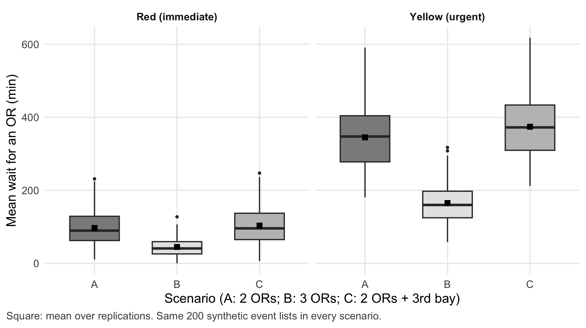
The scenario. After an alert at time zero, 14 casualties who need urgent surgery arrive within three hours. About 40% are triaged red (immediate), the rest yellow (urgent but able to wait). Each patient first occupies one of two resuscitation bays for about 30 minutes and then waits for an operating room. Operations take about two hours for red and one and a half hours for yellow patients, with considerable spread. Red patients have priority at every step. Three scenarios are compared: A, two operating rooms (the regular night set-up); B, three operating rooms; C, two operating rooms and a third resuscitation bay. All numbers are assumptions for teaching. A real plan would take them from the hospital’s own records and from published series.
Fix the events before comparing. The most important design decision comes before any simulation is run. For each of 200 replications, the list of arrival times, triage categories and treatment times is drawn once and stored. All three scenarios then run on exactly the same lists. Differences between scenarios can only come from the capacity, not from one scenario happening to receive sicker patients. In the lab this pairing makes the spread of the estimated difference between A and B about 2.7 times smaller than with independent draws.
| Scenario | Wait for OR, red | Wait for OR, yellow | Wait for bay | Operations within 6 h | Last operation ends (h) |
|---|---|---|---|---|---|
| A: 2 ORs, 2 bays | 97 (25–190) | 345 (222–475) | 26 (11–49) | 4.4 (3–6) | 13.9 |
| B: 3 ORs, 2 bays | 45 (12–90) | 165 (92–244) | 26 (11–49) | 6.5 (5–9) | 10.1 |
| C: 2 ORs, 3 bays | 103 (23–201) | 374 (247–501) | 6 (1–16) | 4.4 (3–6) | 14.0 |
Which resource limits care here? In this scenario the operating rooms do. A third operating room roughly halves the waiting time of yellow patients (from 345 to 165 minutes on average) and finishes the last operation about 3.9 hours earlier. A third resuscitation bay removes most of the waiting for a bay but does not shorten the wait for an operating room; patients simply reach the operating room queue sooner and wait there instead. This is the typical behaviour of a system with one binding constraint: relieving another step moves the queue rather than removing it.
The most important assumption. The comparison holds only for the arrival pattern, treatment times and priority rules written into the model. The simulation shows the consequences of these assumptions; it does not show that the real hospital behaves this way. A published discrete-event model of urban bombing incidents, built from data of 12 incidents, found the resuscitation rooms and the CT scanner, not the operating rooms, to be the main bottlenecks for critical casualties (Hirshberg et al. 1999). That is not a contradiction. Our model has no CT step and only two bays with short occupancy; with other assumptions the binding resource changes. A follow-up model defined surge capacity as a rate of critical casualties per hour rather than a number of beds, about 4.6 per hour with immediately available assets in the studied trauma centre (Hirshberg et al. 2005). Such published figures are useful for a plausibility check of inputs and outputs, not as a validation of a different hospital.
Who carries the waiting? Averages hide the distribution. The priority rule means that yellow patients carry most of the waiting in every scenario; in scenario A, one in ten replications has a 90th-percentile yellow wait above 9.7 hours. A yellow patient who waits that long may deteriorate, which this model does not represent. Scenario B has costs that fall outside the model: the elective operations cancelled in the third room (an assumption of four per activation) and a second on-call team that will be tired the next day. A complete answer to the surgeon names all three groups.
Question for the workshop: Your group gets the same event lists but a plan with three bays and three operating rooms. Before simulating, write down which resource you expect to bind, which patients will carry most of the waiting, and which group outside the model carries a cost.
18.3 Lab
The lab builds the model in five steps: fixed event lists, the model, a verification against a hand calculation, the scenario runs with checks of resource release, and a summary with variation between runs.
NoteR start command
From the root of the book repository, render the chapter (this runs all code, including the figures of the core reading):
quarto render chapters/b18-mass-casualty-capacity-simulation.qmd --to htmlTo run only the Lab code in a fresh R session, start from the chapters/ folder:
Rscript -e 'source(knitr::purl("b18-mass-casualty-capacity-simulation.qmd", output = tempfile(fileext = ".R"), quiet = TRUE))'The chapter writes the fixed event lists to data/b18-event-list.csv; the same file is the shared input for any re-implementation.
18.3.1 Step 1: draw and store the event lists
set.seed(1818)
R_rep <- 200                                   # replications
make_events <- function(rep, n = 14) {
  red <- runif(n) < 0.4                        # triage: 40% red (immediate), rest yellow
  data.frame(
    rep = rep, patient = seq_len(n),
    time = round(sort(runif(n, 0, 180)), 1),   # arrival, minutes after alert (3-hour window)
    triage = ifelse(red, "red", "yellow"),
    priority = ifelse(red, 2L, 1L),            # simmer: higher number is served first
    bay_min = round(rlnorm(n, log(30), 0.3), 1),                          # resuscitation bay time
    or_min = round(rlnorm(n, log(ifelse(red, 120, 90)), 0.35), 1)         # operating time
  )
}
events <- do.call(rbind, lapply(seq_len(R_rep), make_events))
events_fingerprint <- digest::digest(events)   # checksum: the lists must not change later
head(events, 4)
#> rep patient time triage priority bay_min or_min
#> 1 1 1 1.8 red 2 25.5 108.9
#> 2 1 2 53.5 yellow 1 34.5 86.3
#> 3 1 3 58.4 yellow 1 37.8 162.8
#> 4 1 4 65.4 yellow 1 29.1 49.1stopifnot(nrow(events) == R_rep * 14, all(events$bay_min > 0), all(events$or_min > 0))
if (dir.exists("../data")) write.csv(events, "../data/b18-event-list.csv", row.names = FALSE)18.3.2 Step 2: the model
Each patient seizes a bay, holds it for the stored bay time, releases it, then seizes an operating room for the stored operating time. The arrivals come from the stored list (add_dataframe), so the model itself draws no random numbers.
library(simmer)
run_scenario <- function(ev, n_or, n_bay = 2) {
  env <- simmer("mass-casualty")
  patient <- trajectory("patient") |>
    seize("bay", 1) |>
    timeout_from_attribute("bay_min") |>
    release("bay", 1) |>
    set_attribute("ready_for_or", function() now(env)) |>   # time the patient joins the OR queue
    seize("or", 1) |>
    set_attribute("or_start", function() now(env)) |>
    timeout_from_attribute("or_min") |>
    release("or", 1)
  env |>
    add_resource("bay", capacity = n_bay) |>
    add_resource("or", capacity = n_or) |>
    add_dataframe("p", patient, ev[, c("time", "bay_min", "or_min", "priority")], mon = 2,
                  col_time = "time", time = "absolute",
                  col_attributes = c("bay_min", "or_min"), col_priority = "priority") |>
    run()
}

# one row per patient with waiting times; arrival "p0" is row 1 of the event list
patient_table <- function(env, ev) {
  arr <- get_mon_arrivals(env)
  att <- get_mon_attributes(env)
  att <- att[att$key %in% c("ready_for_or", "or_start"), c("name", "key", "value")]
  att <- reshape(att, idvar = "name", timevar = "key", direction = "wide")
  arr <- merge(arr, att, by = "name")
  arr$row <- as.integer(sub("^p", "", arr$name)) + 1
  arr <- arr[order(arr$row), ]
  arr$triage <- ev$triage[arr$row]
  arr$wait_bay <- round(arr$value.ready_for_or - arr$start_time - ev$bay_min[arr$row], 6)
  arr$wait_or <- round(arr$value.or_start - arr$value.ready_for_or, 6)
  arr
}
18.3.3 Step 3: verification against a hand calculation
Before trusting the model with 200 replications, it must reproduce a case that can be computed on paper. Three patients arrive at minutes 0, 1 and 2; there is one bay (10 minutes each) and one operating room (60 minutes each). Patient 3 is red. By hand: patient 1 uses the bay from 0 to 10 and the operating room from 10 to 70 (wait 0). At minute 10 the red patient 3 jumps the bay queue (bay 10 to 20) and waits for the operating room from 20 to 70 (wait 50). Patient 2 uses the bay from 20 to 30 and waits until patient 3 is finished at 130 (wait 100).
hand <- data.frame(time = c(0, 1, 2), bay_min = 10, or_min = 60, priority = c(1L, 1L, 2L),
                   triage = c("yellow", "yellow", "red"))
hand_env <- run_scenario(hand, n_or = 1, n_bay = 1)
hand_tab <- patient_table(hand_env, hand)
hand_tab[, c("name", "triage", "start_time", "value.ready_for_or", "value.or_start", "wait_or", "end_time")]
#> name triage start_time value.ready_for_or value.or_start wait_or end_time
#> 1 p0 yellow 0 10 10 0 70
#> 2 p1 yellow 1 30 130 100 190
#> 3 p2 red 2 20 70 50 130stopifnot(all(hand_tab$wait_or == c(0, 100, 50)), # hand calculation
all(hand_tab$end_time == c(70, 190, 130)))18.3.4 Step 4: run the scenarios and check resource release
For every run, four checks are made: every patient finished; arrival times equal the stored list; at the end both resources are free and their queues empty (no patient kept a resource it should have released); and the area under the operating-room queue-length curve equals the sum of all individual waits for an operating room. The last check is an exact accounting identity behind Little’s law (Little 1961): time spent waiting, counted per patient or counted per minute of queue, must be the same.
run_metrics <- function(ev, n_or, n_bay = 2) {
  env <- run_scenario(ev, n_or, n_bay)
  a <- patient_table(env, ev)
  r <- get_mon_resources(env)
  r <- r[order(r$time), ]
  final <- aggregate(cbind(server, queue) ~ resource, r, function(x) tail(x, 1))
  r_or <- r[r$resource == "or", ]
  queue_area <- sum(head(r_or$queue, -1) * diff(r_or$time))   # integral of OR queue length
  stopifnot(nrow(a) == nrow(ev), all(a$finished),               # everyone finished
            isTRUE(all.equal(a$start_time, ev$time)),           # inputs used unchanged
            all(final$server == 0), all(final$queue == 0),      # resources released
            isTRUE(all.equal(queue_area, sum(a$wait_or))))      # accounting identity
  c(wait_or_red = mean(a$wait_or[a$triage == "red"]),
    wait_or_yellow = mean(a$wait_or[a$triage == "yellow"]),
    p90_yellow = unname(quantile(a$wait_or[a$triage == "yellow"], 0.9)),
    wait_bay = mean(a$wait_bay),
    done_6h = sum(a$end_time <= 360),
    makespan = max(a$end_time))
}
scenarios <- list(A = c(n_or = 2, n_bay = 2), B = c(n_or = 3, n_bay = 2), C = c(n_or = 2, n_bay = 3))
# lists with no yellow patient give NaN for yellow waits; they are kept and reported
b18_res <- lapply(scenarios, function(s)
  t(sapply(seq_len(R_rep), function(r) run_metrics(events[events$rep == r, ], s["n_or"], s["n_bay"]))))
stopifnot(identical(digest::digest(events), events_fingerprint))   # same events in every scenario

b18_mean <- t(sapply(b18_res, colMeans, na.rm = TRUE))
b18_q <- t(sapply(b18_res, function(m) c(apply(m, 2, quantile, 0.05, na.rm = TRUE),
                                          p90_yellow_top10 = unname(quantile(m[, "p90_yellow"], 0.9, na.rm = TRUE)))))
fmt <- function(s, v, d = 0) sprintf("%s (%s–%s)", round(b18_mean[s, v], d),
                                       round(quantile(b18_res[[s]][, v], 0.05, na.rm = TRUE), d),
                                       round(quantile(b18_res[[s]][, v], 0.95, na.rm = TRUE), d))
b18_table <- data.frame(
  scenario = c("A: 2 ORs, 2 bays", "B: 3 ORs, 2 bays", "C: 2 ORs, 3 bays"),
  red = sapply(names(scenarios), fmt, v = "wait_or_red"),
  yellow = sapply(names(scenarios), fmt, v = "wait_or_yellow"),
  bay = sapply(names(scenarios), fmt, v = "wait_bay"),
  done = sapply(names(scenarios), fmt, v = "done_6h", d = 1),
  last = sapply(names(scenarios), function(s) sprintf("%.1f", b18_mean[s, "makespan"] / 60))
)
round(b18_mean, 1)
#> wait_or_red wait_or_yellow p90_yellow wait_bay done_6h makespan
#> A 96.8 345.0 469.2 26.4 4.4 836.7
#> B 44.9 165.2 250.0 26.4 6.5 604.7
#> C 103.4 374.2 512.2 6.2 4.4 837.7# statements made in the core reading
stopifnot(b18_mean["B", "wait_or_yellow"] < 0.6 * b18_mean["A", "wait_or_yellow"], # third OR helps
b18_mean["C", "wait_bay"] < 0.5 * b18_mean["A", "wait_bay"], # third bay removes bay waits
b18_mean["C", "wait_or_yellow"] >= b18_mean["A", "wait_or_yellow"]) # ... but not OR waits18.3.5 Step 5: variation between runs, paired and unpaired
The table in the core reading reports the spread across replications. The more important spread for the decision is that of the difference between scenarios. With paired event lists, each replication gives one difference B minus A for the same 14 patients. For comparison, scenario B is also run on a second, independent set of event lists.
diff_paired <- b18_res$B[, "wait_or_yellow"] - b18_res$A[, "wait_or_yellow"]
set.seed(1819)
events_independent <- do.call(rbind, lapply(seq_len(R_rep), make_events))
res_B_independent <- t(sapply(seq_len(R_rep), function(r)
  run_metrics(events_independent[events_independent$rep == r, ], n_or = 3)))
diff_unpaired <- res_B_independent[, "wait_or_yellow"] - b18_res$A[, "wait_or_yellow"]
b18_sd <- c(paired = sd(diff_paired, na.rm = TRUE), unpaired = sd(diff_unpaired, na.rm = TRUE))
b18_sd_ratio <- unname(b18_sd["unpaired"] / b18_sd["paired"])
round(c(mean_paired = mean(diff_paired, na.rm = TRUE), b18_sd, ratio = b18_sd_ratio), 1)
#> mean_paired paired unpaired ratio
#> -179.9 39.4 105.4 2.7stopifnot(b18_sd["paired"] < b18_sd["unpaired"],
mean(diff_paired < 0, na.rm = TRUE) > 0.95) # B shortens the yellow wait in almost every listWith paired lists, scenario B shortens the mean yellow wait in 100.0% of replications, by 180 minutes on average. The standard deviation of the difference is 39 minutes with paired lists and 105 minutes with independent lists. Pairing does not change what the model assumes; it removes noise that has nothing to do with the question.
NoteOther implementation: SimPy
Original implementation. SimPy, a process-based discrete-event simulation library for Python (Team SimPy, n.d.), version 4.1.2 (current release on the Python Package Index, accessed 8 November 2026); documentation.
Concrete advantage. Each patient is written as a Python generator function, so interruptions, pre-emption and re-triage can be followed line by line in the program flow. Teams with an existing Python data pipeline can keep the simulation in the same environment.
What must be identical for a fair comparison. The input file data/b18-event-list.csv (arrival, triage, bay and operating times per replication), the capacities, and the priority rule. Note the direction: in simmer a higher priority number is served first, in SimPy’s PriorityResource a lower number is. Ties are resolved by the time of the request in SimPy; check that equal arrival times are ordered the same way. Compare the event log (order of starts and ends) first, then the waiting times. Tolerance: identical event order and waiting times equal up to floating-point rounding (10⁻⁶ minutes). The same seed in R and Python does not produce the same random draws, which is why the event list is exchanged as a file rather than regenerated.
Status. Conceptual comparison, not executed. No statement about speed is made.
18.4 Counter-check
Scenario C, the third resuscitation bay, is the counter-check. Before looking at the numbers, predict: will the mean wait for a bay go up or down? Will the mean wait for an operating room go up, down or stay the same? Then compare with the code output.
round(rbind(A = b18_mean["A", c("wait_bay", "wait_or_red", "wait_or_yellow", "makespan")],
            C = b18_mean["C", c("wait_bay", "wait_or_red", "wait_or_yellow", "makespan")]), 1)
#> wait_bay wait_or_red wait_or_yellow makespan
#> A 26.4 96.8 345.0 836.7
#> C 6.2 103.4 374.2 837.7stopifnot(abs(b18_mean["C", "makespan"] - b18_mean["A", "makespan"]) < 15) # last operation hardly movesThe wait for a bay falls from 26 to 6 minutes, but the wait for an operating room does not fall; for yellow patients it rises slightly (345 to 374 minutes), because patients now reach the operating room queue earlier and wait there instead, while the two operating rooms work through the same caseload at the same pace. The time until the last operation ends hardly changes. In this scenario the third bay buys comfort in the emergency department, not earlier surgery. Change one more assumption yourself: shorten the bay time to 15 minutes, or add a CT step with one scanner, and check whether the binding resource moves.
18.5 Consequences for patients and operations
Ethics. A triage rule is a value judgement about who waits. The model makes its consequences visible: in every scenario yellow patients carry most of the waiting, and the model does not represent deterioration while waiting, which would turn some yellow patients red. Capacity decisions also distribute burdens outside the model: elective patients whose operations are cancelled, and the on-call team that works through the night. A mass casualty plan that reports only the mean waiting time of casualties leaves these groups out; Chapter 21 discusses how to make such trade-offs explicit.
Reporting and validity. Simulation studies should report inputs, their sources, the handling of random numbers, the number of replications and the verification steps; the STRESS guidelines give a checklist (Monks et al. 2019). A plan based on a simulation should state which inputs were assumptions and which came from local data, and when they will be checked against the next exercise or real incident.
Regulation. Indirect. A planning simulation for a mass casualty plan has no medical purpose for an individual patient. The question changes if software is used during an incident to assign individual patients to operating rooms or to set treatment priority. Systems for emergency healthcare patient triage are listed as high-risk uses in Annex III, point 5(d), of the AI Act (European Parliament and Council of the European Union 2024); for such a use the questions of Chapter 22 apply. As of November 2026.
Data protection and security. Treatment times derived from the hospital’s operating-room records are health data when they are linked to persons; for the model, aggregated distributions per procedure group are sufficient. During a real incident, the plan must work if scheduling software is unavailable; a printed version of the decision rules is part of the fallback (Chapter 24).
18.6 Look up and transfer
- Reviewer question: Were the scenarios compared on identical input events, how many replications were run, how was the model verified, and which inputs are local data and which are assumptions?
- Self-test: A team compares two and three operating rooms with 50 replications per scenario. Each scenario uses its own random seed. They report mean yellow waits of 410 and 200 minutes with overlapping 95% intervals across replications and conclude that “the difference is uncertain”. What would you change in the design and in the report?
TipAnswer
Draw the event lists once and run both scenarios on the same lists (common random numbers). Report the distribution of the paired differences per replication, for example the mean difference with its 5th and 95th percentiles and the share of replications in which three rooms are better. Overlapping intervals of two separate means are the wrong comparison: most of their width comes from differences between event lists, which affect both scenarios alike. Also report the waits of red and yellow patients separately and name the costs outside the model (cancelled elective operations, staff).
- Annotated sources:
- Ucar et al. (2019) describe
simmer, the discrete-event simulation package used in the lab; the simmer website documentsadd_dataframe()and the monitoring functions. - Sargent (2013) summarises verification and validation of simulation models, including the difference between checking the model logic and checking the model against reality.
- Monks et al. (2019) (STRESS) provide reporting guidelines for simulation studies.
- Hirshberg et al. (1999) built a discrete-event model of hospital resources in urban bombing incidents and found resuscitation rooms and CT, not operating rooms, to be the bottlenecks for critical casualties.
- Hirshberg et al. (2005) related casualty load to the level of trauma care and expressed surge capacity as a rate of critical casualties per hour.
- Little (1961) proved the queuing formula L = λW, which underlies the accounting check in step 4.
- Team SimPy (n.d.) is the documentation of SimPy for the comparison box.
- Ucar et al. (2019) describe
In W6 (teaching unit 22, station “mass casualty”) learners simulate paired arrival sequences for two capacity scenarios and hand in a waiting-time distribution with its spread across runs. The project work in teaching unit 24 uses the same structure: model, baseline scenario and one counter-check that another group reproduces from a fresh R session.
18.7 Further reading
- Chapter 17 for the forecast that often supplies the arrival assumptions of a capacity simulation.
- Chapter 15 for the other simulation type in W6, a mechanistic model checked against an analytical solution.
- Chapter 21 for the ethics of triage and of distributing waiting between patient groups.
- Chapter 27 for reporting a simulation in a model passport.
- Strategy in R: Agent-Based Models for Strategic Interaction for models in which individuals adapt their behaviour.
- Strategy in R: Probability Essentials, law of large numbers and Monte Carlo for why more replications narrow the estimate of a mean but not the spread between runs.
- Methods in R cheat sheet: Power by simulation for the same replicate-and-summarise pattern in study planning.