16 Bayes, small samples and the 3Rs
R. Heller · Date: 2025-06-15 · Last changed: 2026-11-09
16.1 Case and decision
A fictitious preclinical group has tested a new bone substitute material in a critical-size femoral defect model in rats. Ten animals were operated on; one died on the second day after surgery; in seven of the nine animals evaluated at week 8, the defect was bridged by bone. There was no control group. The draft abstract reads: “The material led to bony bridging in 78% of animals and is therefore effective.” The group leader has to decide two things before the manuscript goes out and before the next application to the competent authority: what the abstract may claim, and which experiment – if any – should come next. All animals and results are synthetic. The chapter separates three questions that the draft merges: how large the bridging rate is, whether the material caused it, and whether another experiment on animals is justified.
16.2 Core reading
Origin and denominator first. The independent unit is the animal (Lazic et al. 2018). Ten were operated on; one died before the end point; nine were evaluated; seven were bridged. The draft reports 7/9 = 77.8%. If the animal that died is counted as a failure, the rate is 7/10 = 70.0%. Both numbers are correct; they answer different questions, and the report must say which one it uses and why. A short table that lists all ten animals with their status is the clearest way to show both. Reporting the excluded animal is not optional: the ARRIVE guidelines list inclusion and exclusion criteria among the “Essential 10” items (Percie du Sert et al. 2020).
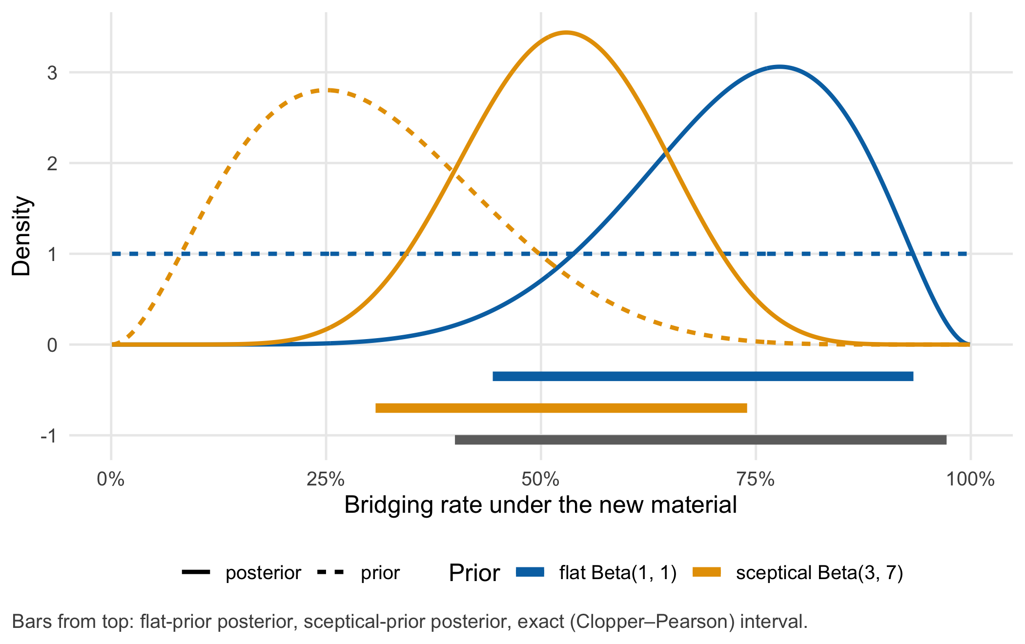
A frequentist baseline. The exact (Clopper–Pearson) 95% confidence interval for 7 of 9 runs from 40.0% to 97.2% (Clopper and Pearson 1934). With nine animals, “78%” is compatible with a rate below one half and with a rate close to one.
Prior, likelihood and posterior. Bayesian analysis asks a slightly different question: given the data, how plausible is each possible bridging rate p? It combines three parts. The likelihood says how probable 7 bridged out of 9 is for each value of p (a binomial model). The prior states what was considered plausible before the experiment. The posterior is the updated belief: prior × likelihood, rescaled. For a binomial outcome and a Beta prior, the posterior is again a Beta distribution: Beta(a, b) becomes Beta(a + 7, b + 2). Its quantiles come from qbeta() without simulation (Spiegelhalter et al. 2004). The prior parameters can be read as imaginary animals observed beforehand: Beta(1, 1) adds one bridged and one unbridged animal, Beta(3, 7) adds three and seven. With only nine real animals, ten imaginary ones carry real weight.
Two priors are plausible here (both assumptions). A flat prior, Beta(1, 1), treats every rate between 0 and 1 as equally plausible. A sceptical prior, Beta(3, 7), expresses the expectation that the material performs about as well as an untreated defect in this model, assumed here to bridge in about 30% of animals, and gives this expectation the weight of ten animals. Figure 16.1 and Table 16.1 show the result.
qbeta() and pbeta().
| Prior | Rationale | Posterior | Mean and 95% interval | P(rate > 50%) |
|---|---|---|---|---|
| flat Beta(1, 1) | every rate equally plausible | Beta(8, 3) | 72.7% (44.4% to 93.3%) | 0.95 |
| sceptical Beta(3, 7) | about 30%, as assumed for untreated defects; weight of 10 animals | Beta(10, 9) | 52.6% (30.8% to 74.0%) | 0.59 |
With the flat prior, the posterior mean is 72.7%, the 95% interval runs from 44.4% to 93.3%, and the probability that the rate exceeds one half is 0.95. With the sceptical prior, the mean falls to 52.6% and that probability to 0.59. Nine animals are not enough to make the prior irrelevant. Reporting both analyses, with the prior chosen before the data were seen, is more informative than reporting either alone. Note the difference in meaning: a posterior interval is a statement about the rate, given the model and the prior; the confidence interval is a statement about how often the procedure would cover the true rate in repeated experiments. With small samples the two can differ noticeably.
The most important assumption. Every interval in this chapter describes the bridging rate under the new material in this model and this laboratory. None of them says what the rate would have been without the material. An effect is a comparison: rate with the material minus rate without it. The second rate was not observed. If an untreated defect bridged in 20% of animals, the posterior probability that the material does better is above 0.999; at 50%, it is 0.95; at 70%, it is 0.62 (flat prior). The data cannot choose between these scenarios, so the claim “is effective” has no support from this experiment. A historical rate from another publication is no substitute for a concurrent, randomised control: animals, surgeons, housing and assessment differ.
What the next experiment needs. A defensible next step answers the question that this experiment could not: does the material change the bridging rate? That requires a concurrent control group in the same model and laboratory, random allocation of animals to groups, outcome assessment by a person who does not know the group, an end point and a sample size fixed before the first operation, and a report of every animal. It also requires a criterion, agreed in advance, under which the experiment is not run – for example when the number of animals that can be justified cannot answer the question with reasonable probability. The lab computes both.
Planning versus reporting. Two frameworks apply, at different moments. The 3Rs – replacement, reduction and refinement – govern whether and how an experiment is done (NC3Rs 2026). In the European Union they are binding on Member States through Article 4 of Directive 2010/63/EU on the protection of animals used for scientific purposes (European Parliament and Council of the European Union 2010). The ARRIVE guidelines 2.0 govern how a completed study is reported (Percie du Sert et al. 2020). Good reporting cannot repair a design without a control group, and a well-planned design is of little use if the report omits the excluded animal.
Question for the workshop. Write one sentence for the abstract that is true for these data and that a sceptical reader would accept. Which word in the draft sentence has to go first?
16.3 Lab
The lab uses base R only (plus ggplot2 for the figure above) and runs in under a second.
16.3.1 Step 1: the data with their origin
animals <- data.frame(
  animal = sprintf("R%02d", 1:10),                                  # fictitious rats
  died_before_end_point = c(FALSE, TRUE, rep(FALSE, 8)),            # R02 died on day 2 after surgery
  bridged_week8 = c(TRUE, NA, TRUE, TRUE, FALSE, TRUE, TRUE, TRUE, FALSE, TRUE))  # NA: not evaluable
n_operated <- nrow(animals)
n_evaluated <- sum(!animals$died_before_end_point)
x_bridged <- sum(animals$bridged_week8, na.rm = TRUE)
stopifnot(n_operated == 10, n_evaluated == 9, x_bridged == 7,
          all(is.na(animals$bridged_week8) == animals$died_before_end_point))  # no evaluation without an animal
16.3.2 Step 2: the frequentist baseline
cp_interval <- binom.test(x_bridged, n_evaluated)$conf.int            # exact Clopper–Pearson interval
cp_interval_operated <- binom.test(x_bridged, n_operated)$conf.int    # death counted as failure
round(rbind(evaluated_7_of_9 = cp_interval, operated_7_of_10 = cp_interval_operated), 3)
#> [,1] [,2]
#> evaluated_7_of_9 0.400 0.972
#> operated_7_of_10 0.348 0.93316.3.3 Step 3: two priors and their posteriors
priors <- data.frame(label = c("flat Beta(1, 1)", "sceptical Beta(3, 7)"), a = c(1, 3), b = c(1, 7),
                     rationale = c("every rate equally plausible",
                                   "about 30%, as assumed for untreated defects; weight of 10 animals"))
posterior_of <- function(x, n, a, b) {                     # conjugate update Beta(a, b) -> Beta(a + x, b + n - x)
  a_post <- a + x
  b_post <- b + n - x
  data.frame(a_post = a_post, b_post = b_post, mean = a_post / (a_post + b_post),
             lower = qbeta(0.025, a_post, b_post), upper = qbeta(0.975, a_post, b_post),
             p_above_half = 1 - pbeta(0.5, a_post, b_post))
}
posterior <- do.call(rbind, Map(posterior_of, x_bridged, n_evaluated, priors$a, priors$b))
prior_interval <- qbeta(c(0.025, 0.975), 3, 7)            # what the sceptical prior allowed beforehand
posterior_table <- data.frame(
  Prior = priors$label, Rationale = priors$rationale,
  Posterior = sprintf("Beta(%d, %d)", posterior$a_post, posterior$b_post),
  `Mean and 95% interval` = sprintf("%s (%s to %s)", cdsr_percent(posterior$mean), cdsr_percent(posterior$lower),
                                    cdsr_percent(posterior$upper)),
  `P(rate > 50%)` = cdsr_number(posterior$p_above_half, 2), check.names = FALSE)
posterior[, -(1:2)] |> round(3)
#> mean lower upper p_above_half
#> 1 0.727 0.444 0.933 0.945
#> 2 0.526 0.308 0.740 0.593stopifnot(
posterior$a_post == c(8, 10), posterior$b_post == c(3, 9),
abs(posterior$lower - c(0.444, 0.308)) < 0.001, abs(posterior$upper - c(0.933, 0.740)) < 0.001,
posterior$upper[2] < posterior$upper[1], # the sceptical prior pulls the interval down
cp_interval[2] - cp_interval[1] > posterior$upper[1] - posterior$lower[1]) # exact interval is the widestThe sceptical prior on its own allowed rates from 7.5% to 60.0%. Its posterior is a compromise between this expectation and the data; with nine animals, neither dominates.
16.3.4 Step 4: event rate is not effect
control_rates <- c(0.2, 0.5, 0.7)                          # hypothetical rates without the material (not observed)
p_beats_control <- 1 - pbeta(control_rates, posterior$a_post[1], posterior$b_post[1])
data.frame(assumed_control_rate = control_rates, P_material_better = round(p_beats_control, 3))
#> assumed_control_rate P_material_better
#> 1 0.2 1.000
#> 2 0.5 0.945
#> 3 0.7 0.617stopifnot(p_beats_control[1] > 0.999, p_beats_control[3] < 0.7) # the answer depends on what was not measured16.3.5 Step 5: design of the next experiment
The next defensible experiment, if any, compares the material with a concurrent control in a randomised design, with the outcome assessed blind to group. Its size follows from a design analysis before any animal is ordered. Here the decision rule is: call the material better if the posterior probability that its rate exceeds the control rate is above 0.95 (flat priors in both arms). For each number of animals per arm, the probability that the rule declares success can be computed exactly by summing over all possible outcomes – no simulation is needed.
prob_better <- function(x_t, x_c, n) {                     # P(p_material > p_control | data), flat priors
  integrate(function(p) dbeta(p, 1 + x_c, 1 + n - x_c) * (1 - pbeta(p, 1 + x_t, 1 + n - x_t)), 0, 1)$value
}
decision_probability <- function(n, p_material, p_control, threshold = 0.95) {
  outcomes <- expand.grid(x_t = 0:n, x_c = 0:n)
  success <- mapply(prob_better, outcomes$x_t, outcomes$x_c, MoreArgs = list(n = n)) > threshold
  sum(dbinom(outcomes$x_t, n, p_material) * dbinom(outcomes$x_c, n, p_control) * success)
}
n_per_arm <- c(6, 8, 10, 12, 15, 20)
design <- data.frame(
  n_per_arm = n_per_arm,
  success_if_relevant_difference = sapply(n_per_arm, decision_probability, p_material = 0.7, p_control = 0.3),
  success_if_no_difference = sapply(n_per_arm, decision_probability, p_material = 0.3, p_control = 0.3))
round(design, 3)
#> n_per_arm success_if_relevant_difference success_if_no_difference
#> 1 6 0.296 0.034
#> 2 8 0.455 0.041
#> 3 10 0.609 0.050
#> 4 12 0.596 0.053
#> 5 15 0.731 0.043
#> 6 20 0.808 0.044n_needed <- min(design$n_per_arm[design$success_if_relevant_difference >= 0.8])
stopifnot(all(design$success_if_no_difference < 0.06), # false-positive probability stays near 5%
n_needed == 20)The assumed relevant difference is 30% versus 70% (assumption). To reach a decision probability of 80%, the binary end point needs 20 animals per arm. The probabilities do not rise smoothly with the number of animals because the outcome is discrete.
A criterion against a further experiment. Fix it before the application, together with the animal welfare body. For example: if the largest number of animals that the team considers justifiable for this question – say 12 per arm (assumption) – gives a decision probability below 80% for the smallest relevant difference, the experiment is not run in this form. Here, 12 per arm give 59.6%, so the criterion applies. The alternatives are not “more animals” but better information per animal and fewer animals overall: a continuous end point such as bone volume from imaging instead of bridged yes/no (reduction), non-animal tests of the material’s properties before any further surgery (replacement, partial), and a revised anaesthesia and analgesia protocol after the early death (refinement).
16.3.6 Step 6: planning and reporting are different tasks
Table 16.2 sets the two frameworks side by side for this case.
| 3Rs | ARRIVE 2.0 | |
|---|---|---|
| Question | Is the experiment necessary, and how can harm and numbers be minimised? | Can readers judge and repeat what was done? |
| When | Before the experiment: design, application, ethical review | After the experiment: manuscript |
| Basis | NC3Rs definitions (NC3Rs 2026); Directive 2010/63/EU, Article 4 (European Parliament and Council of the European Union 2010) | Essential 10 and Recommended Set (Percie du Sert et al. 2020) |
| In this case | Concurrent control, design analysis, continuous end point, refined anaesthesia | Report all 10 animals, the death and its handling, the absent control and blinding |
The ARRIVE “Essential 10” are study design, sample size, inclusion and exclusion criteria, randomisation, blinding, outcome measures, statistical methods, experimental animals, experimental procedures and results. In a survey of 271 publications of animal research, most studies did not use randomisation (87%) or blinding (86%), and only 59% stated the objective together with the number and characteristics of the animals (published, Kilkenny et al. (2009)).
16.3.7 Step 7: decision exercise – a letter to the editor
Assume the draft sentence was published unchanged. Write a letter to the editor of about 150 words that explains, for a clinical readership, the difference between the observed bridging rate and a treatment effect. Use the denominators, one interval and one consequence for the next study. Compare your letter with the example only after writing it.
TipExample letter
The authors report bony bridging in 78% of rats treated with a new bone substitute and conclude that the material is effective. We would like to raise two points. First, ten animals were operated on and one died; the rate is 7/9, or 7/10 if the death is counted. The exact 95% confidence interval for 7/9 runs from 40% to 97%. Second, and more important, there was no control group. Whether 78% is better than what an untreated defect achieves in this model, operated and assessed in the same laboratory, is unknown; historical rates from other studies cannot answer this. The data therefore describe how often bridging occurred, not whether the material caused it. A randomised experiment with a concurrent control, blinded assessment and a sample size justified in advance would be needed before any claim of efficacy, and before planning studies in patients.
If the result stays unclear. A small single-arm experiment with an unclear result is still worth reporting – with all animals, both denominators and the absent control stated plainly – because unreported experiments lead others to repeat them. Its legitimate use is to inform the design of the next experiment: it suggests a plausible range for the treated rate, as in the sceptical-prior analysis, not a proof of effect.
16.4 Counter-check
Triple the number of animals and keep the rate: 21 bridged of 27 evaluated (synthetic). Predict first: will the two posteriors move closer together? Will the uncertainty about the effect of the material shrink?
posterior_27 <- do.call(rbind, Map(posterior_of, 21, 27, priors$a, priors$b))
widths <- data.frame(prior = priors$label,
                     width_9 = posterior$upper - posterior$lower,
                     width_27 = posterior_27$upper - posterior_27$lower,
                     mean_9 = posterior$mean, mean_27 = posterior_27$mean)
round(widths[, -1], 3)
#> width_9 width_27 mean_9 mean_27
#> 1 0.489 0.303 0.727 0.759
#> 2 0.432 0.301 0.526 0.649gap_9 <- diff(posterior$mean); gap_27 <- diff(posterior_27$mean)
stopifnot(all(widths$width_27 < widths$width_9), # intervals narrow
abs(gap_27) < abs(gap_9)) # the priors matter lessThe intervals narrow, and the difference between the posterior means under the two priors shrinks from 20.1 to 11.0 percentage points. The uncertainty about the rate falls. The uncertainty about the effect does not change at all, because 27 treated animals without a control still contain no information about the rate without treatment. Tripling the number of animals in an uncontrolled design costs animals without answering the question – the opposite of reduction in the sense of the NC3Rs, which ties reduction to appropriately designed experiments that add to the knowledge base (NC3Rs 2026).
16.5 Consequences for patients and operations
Animals and ethics. Each further animal needs a justification that this design cannot supply. The early death is a signal for refinement before any further surgery, and the criterion against a further experiment protects animals from a study that could not answer its question. In Germany, the Animal Welfare Act (Tierschutzgesetz, TierSchG) § 7a requires that animal experiments are indispensable for their purpose and, for vertebrates and cephalopods, ethically justifiable with respect to the expected pain, suffering or harm (Federal Republic of Germany 2006).
Law: what binds whom (as of November 2026). Directive 2010/63/EU was adopted on 22 September 2010, published in the Official Journal on 20 October 2010 and entered into force on 9 November 2010; Member States had to transpose it by 10 November 2012 and apply their rules from 1 January 2013 (European Parliament and Council of the European Union 2010). Article 4 (replacement, reduction, refinement) addresses Member States and reaches researchers through national law; later amendments (Regulation (EU) 2019/1010 and Delegated Directive (EU) 2024/1262) changed reporting rules and annexes, not Article 4. The NC3Rs definitions of the 3Rs and the ARRIVE guidelines are guidance, not law, although journals and funders may make ARRIVE reporting a condition. Whether the next experiment needs a new project authorisation or an amendment, and which authority decides, is a local question for the animal welfare officer and the competent authority (open).
Patients. A claim of efficacy from an uncontrolled animal series can travel into grant applications and early clinical plans. If the material were developed for patients, its preclinical evidence would become part of the evidence assessed under medical device rules (Chapter 22, interpretation); a misleading abstract weakens that chain from the start.
Data and security. Indirect: the animal-level data, including the excluded animal, should be stored with the protocol so that the denominators can be reconstructed (Chapter 4, Chapter 27).
16.6 Look up and transfer
Reviewer question. Which animals were operated, excluded and evaluated, was there a concurrent randomised control group, and how sensitive are the conclusions to the prior?
Self-test. In a second fictitious model, 0 of 8 treated animals develop a wound infection. A colleague writes “the material prevents infection (0%)”. Compute a 95% posterior interval under a flat prior and explain what the result can and cannot support.
TipAnswer
The posterior is Beta(1, 9). Its 95% interval is qbeta(c(0.025, 0.975), 1, 9), about 0.3% to 33.6%; with the one-sided “upper 95% bound”, qbeta(0.95, 1, 9) gives about 28%. Zero events in eight animals are compatible with an infection rate of more than one in four. And as in the case, without a control group the data say nothing about prevention: infection might be rare in this model anyway.
Annotated sources.
- Spiegelhalter et al. (2004) – Bayesian reasoning for trials and health-care evaluation, including the choice and reporting of priors.
- Clopper and Pearson (1934) – the exact binomial confidence interval used as the frequentist baseline.
- Lazic et al. (2018) – what counts as the independent unit (“N”) in animal experiments.
- Percie du Sert et al. (2020) – the ARRIVE guidelines 2.0 for reporting animal research.
- NC3Rs (2026) – current definitions of replacement, reduction and refinement.
- European Parliament and Council of the European Union (2010) – the binding EU framework, including Article 4 on the 3Rs.
- Federal Republic of Germany (2006) – the German provision on the indispensability and ethical justifiability of animal experiments.
- Kilkenny et al. (2009) – evidence of reporting and design gaps in published animal research.
16.7 Further reading
- Chapter 19 – what changes when a result is transferred from one species or centre to the next.
- Chapter 27 – reporting templates for animal studies within the model passport.
- Methods in R: The Beta-Binomial Model and Prior Specification – the conjugate model of this chapter and how to choose and justify priors.
- Methods in R: ARRIVE – animal research – a reporting template for the items discussed here.
- CTTIR Course 3, Week 1, Session 4 – Bench and translational design – designing preclinical experiments with controls and randomisation.
- CTTIR Course 4, Week 3, Session 1 – Bayesian thinking; α control vs decision error – decision rules based on posterior probabilities.
- CTTIR Tutorials: Credible Intervals – equal-tailed and highest-density intervals.