13 Longitudinal biomarkers
R. Heller · Date: 2025-03-30 · Last changed: 2026-11-09
13.1 Case and decision
A doctoral researcher in a fictitious spinal cord injury centre has serum selenium values from 36 people after traumatic spinal cord injury: one sample at admission and up to five more over the following eight weeks. Before the next research meeting, the supervising consultant asks a single question. Does selenium recover more slowly after a complete injury than after an incomplete one? If it does, the team will draft a protocol for a supplementation trial restricted to people with complete injuries. Published observational work on trace elements after spinal cord injury motivates the question (Seelig et al. 2020); every value in this chapter is synthetic. Not everybody stayed for all visits. Some people were transferred, others missed late appointments. Whether the protocol is justified therefore depends on a question that sounds technical but is clinical: whose course does the estimated slope describe?
13.2 Core reading
One table, three levels. A longitudinal data set has three levels that are easily confused: the person, the visit and the measurement. Here, 36 people (18 per injury group) were due to be sampled six times, at admission and at weeks 1, 2, 4, 6 and 8. That gives 216 planned values; 186 were measured. The independent unit is the person. Any statement about “the course after a complete injury” is a statement about people, so its uncertainty must be driven by the number of people, not by the number of tubes in the freezer.
The quantity of interest. The consultant’s question concerns a time–group interaction: the difference between the mean change per week after a complete injury (ASIA Impairment Scale grade A) and after an incomplete injury (grades B–D). Its unit is µg/L per week. A value of −1 means that selenium rises by 1 µg/L per week less after a complete injury. The difference at admission is a separate quantity, the group main effect, and answers a different question.
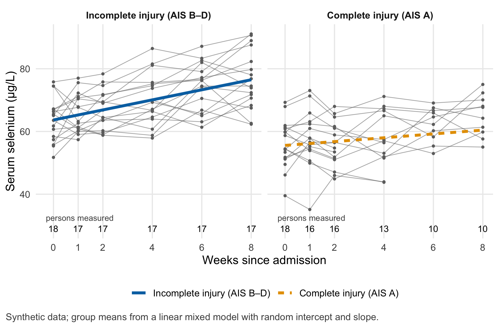
What the figure shows. Figure 13.1 draws one thin line per person (a spaghetti plot) and the fitted mean course of each group. In the complete-injury group, the denominator falls from 18 at admission to 10 at week 8; in the incomplete group it falls to 17. People with low values left more often. The people still visible at week 8 are therefore not a random subset of those admitted.
Three answers to one question. Table 13.1 compares three ways of estimating the interaction.
- Pooled regression. One straight line per group through all measured values, as if every measurement came from a different person. It ignores that values from the same person are correlated, so its interval is too narrow for a statement about people, and it lets persons with many visits dominate. Here, the late visits come mostly from people with a better course, and the estimated difference shrinks towards zero.
- Slope per person (baseline). For each person with at least two values, fit a straight line and keep its slope; then compare the mean slope between groups. This summary-measure approach (Matthews et al. 1990) is the biometrically sensible baseline: transparent, person-based and easy to check by hand. It weights a person with two values like a person with six, and it silently drops people with a single value.
- Linear mixed model. A model with a random intercept and a random slope per person (Laird and Ware 1982), fitted with lme4 (Bates et al. 2015). Each person gets their own line, but lines from people with few values are pulled towards the group mean. All 36 persons and all measured values enter.
| Approach | Units used | Difference | Lower 95% | Upper 95% |
|---|---|---|---|---|
| Pooled regression (ignores persons) | 186 measurements | -0.54 | -1.33 | 0.25 |
| Slope per person (baseline) | 33 persons | -1.13 | -1.92 | -0.34 |
| Mixed model, random intercept and slope | 36 persons, 186 measurements | -0.99 | -1.67 | -0.31 |
| Simulation truth | 36 persons, 216 planned values | -1.00 |
Because the data are synthetic, the true difference (−1.0 µg/L per week) is known. In this cohort, the pooled regression underestimates the difference, the per-person slopes overestimate it and the mixed model comes closest. One cohort proves nothing about a method; the counter-check repeats the experiment a hundred times (Section 13.4).
Whose course? The three numbers describe different people. The pooled slope is the course of the measurements, and late measurements come from those who stayed. The mean of per-person slopes describes everybody with at least two values, each counted once, however noisy their line. The fixed slope of the mixed model describes a typical admitted person – under one condition.
The most important assumption. The mixed model’s slope describes everyone who was admitted only if the chance of leaving the study depends on what had already been measured, not on the unmeasured current value or on the person’s own unobserved rate of recovery. This condition is called missing at random (MAR) (Rubin 1976). In the simulation, transfers depend on the last measured selenium value, a stand-in for the observable clinical condition, so MAR holds by construction. In a real cohort, it is an assumption that no analysis of the observed data can prove. When leaving depends on what was not observed (missing not at random, MNAR), every estimate in Table 13.1 can be biased, and the honest response is a sensitivity analysis (Diggle and Kenward 1994; Little et al. 2012). The mechanisms are explained in more depth in the Methods in R lab on MCAR, MAR and MNAR.
What to say in the meeting. A defensible sentence would be: “In 36 people, selenium rose by about 1.0 µg/L per week less after a complete injury (mixed model, 95% CI 0.3 to 1.7). This assumes that leaving the study depended on observed values. If the people who left had values about 18 µg/L higher than their own earlier course predicts, the difference would disappear.” The last sentence comes from the sensitivity analysis in the lab. It turns a hidden assumption into a number that the clinical team can judge.
Question for the workshop. Which observable reason for leaving the study – transfer to intensive care, death, discharge home, a missed outpatient appointment – would make the MAR assumption more plausible, and which less? Sort the four reasons before you open the lab.
13.3 Lab
The lab runs in a fresh R session in about ten seconds. It needs lme4 and ggplot2.
13.3.1 Step 1: write down the simulation assumptions
Every number in the simulation is an assumption that is set here and nowhere else. The dropout rule makes the chance of leaving before the next visit depend on the last measured value (MAR). A second rule, used only in the counter-check, makes it depend on the unmeasured current level and on the person’s own recovery rate (MNAR).
set.seed(1313)                                     # set again so this chunk always gives the same cohort
n_per_group <- 18                                  # persons per injury group
weeks <- c(0, 1, 2, 4, 6, 8)                       # planned visits, weeks since admission
true_start <- c(incomplete = 62, complete = 58)    # mean selenium at admission (µg/L)
true_slope <- c(incomplete = 1.6, complete = 0.6)  # mean change (µg/L per week)
sd_start <- 7                                      # between-person SD at admission (µg/L)
sd_slope <- 0.6                                    # between-person SD of the weekly change (µg/L per week)
sd_noise <- 4                                      # measurement and day-to-day noise (µg/L)

simulate_cohort <- function(mechanism = c("mar", "mnar", "none")) {
  mechanism <- match.arg(mechanism)
  ids <- sprintf("P%02d", seq_len(2 * n_per_group))
  group <- rep(names(true_start), each = n_per_group)
  dev_start <- rnorm(length(ids), 0, sd_start)     # each person's deviation at admission
  dev_slope <- rnorm(length(ids), 0, sd_slope)     # each person's deviation of the weekly change
  d <- data.frame(id = rep(ids, each = length(weeks)),
                  group = rep(group, each = length(weeks)),
                  week = rep(weeks, times = length(ids)))
  p <- match(d$id, ids)
  d$true_level <- true_start[d$group] + dev_start[p] + (true_slope[d$group] + dev_slope[p]) * d$week
  d$selenium <- d$true_level + rnorm(nrow(d), 0, sd_noise)
  d$observed <- TRUE
  for (k in seq_along(ids)) {                      # monotone dropout: once gone, always gone
    r <- which(d$id == ids[k])
    for (j in 2:length(r)) {
      linear_predictor <- switch(mechanism,
        none = -Inf,
        mar  = -2.8 - 0.2 * (d$selenium[r[j - 1]] - 60),               # last measured value
        mnar = -2.8 - 0.2 * (d$true_level[r[j]] - 60) - 1.5 * dev_slope[k] / sd_slope)  # unmeasured state
      if (runif(1) < plogis(linear_predictor)) {
        d$observed[r[j:length(r)]] <- FALSE
        break
      }
    }
  }
  d$group <- factor(d$group, levels = c("incomplete", "complete"))
  d
}

cohort_full <- simulate_cohort("mar")              # all planned visits, with the observed flag
cohort <- cohort_full[cohort_full$observed, c("id", "group", "week", "selenium")]
n_persons <- length(unique(cohort$id))
n_week8 <- table(cohort$group[cohort$week == 8])   # persons still measured at week 8
stopifnot(nrow(cohort_full) == 216, n_persons == 36,
          all(table(cohort$id[cohort$week == 0]) == 1))  # everybody has an admission value
13.3.2 Step 2: document the denominators at person level
Before any model, count people, not rows. Table 13.2 gives the denominator for every visit and the number of people who contribute at least two values (needed for a per-person slope).
per_visit <- as.data.frame.matrix(table(cohort$group, cohort$week))
n_meas_person <- table(cohort$id)
group_of_id <- tapply(as.character(cohort$group), cohort$id, unique)
per_visit$`persons with ≥ 2 values` <- as.vector(tapply(n_meas_person >= 2, group_of_id, sum)[rownames(per_visit)])
per_visit$`all measurements` <- as.vector(table(cohort$group)[rownames(per_visit)])
names(per_visit)[1:6] <- paste("week", weeks)
knitr::kable(per_visit)| week 0 | week 1 | week 2 | week 4 | week 6 | week 8 | persons with ≥ 2 values | all measurements | |
|---|---|---|---|---|---|---|---|---|
| incomplete | 18 | 17 | 17 | 17 | 17 | 17 | 17 | 103 |
| complete | 18 | 16 | 16 | 13 | 10 | 10 | 16 | 83 |
stopifnot(per_visit$`week 0` == c(18, 18),                 # nobody is missing at admission
          sum(per_visit$`all measurements`) == nrow(cohort))
The data set is saved for the workshop; it contains only the synthetic values that this chapter generates.
write.csv(cohort, "../data/b13-selenium-synthetic.csv", row.names = FALSE)13.3.3 Step 3: three estimates of the interaction
library(lme4)
ctrl <- lmerControl(optimizer = "bobyqa")
# (1) Pooled regression: every measurement treated as if it were a separate person (a common mistake)
fit_pooled <- lm(selenium ~ week * group, data = cohort)

# (2) Baseline: one least-squares slope per person with at least two values
per_person <- do.call(rbind, lapply(split(cohort, cohort$id), function(d) {
  if (nrow(d) < 2) return(NULL)
  data.frame(id = d$id[1], group = d$group[1], n_values = nrow(d),
             slope = unname(coef(lm(selenium ~ week, data = d))["week"]))
}))
welch <- t.test(slope ~ group, data = per_person)   # Welch test; estimates are incomplete, complete

# (3) Linear mixed model: random intercept and random slope for every person
fit_lmm <- lmer(selenium ~ week * group + (week | id), data = cohort, REML = TRUE, control = ctrl)
summary(fit_lmm)$coefficients
#> Estimate Std. Error t value
#> (Intercept) 63.6672802 1.5549898 40.943856
#> week 1.6025084 0.2190990 7.314082
#> groupcomplete -8.1093780 2.2107273 -3.668195
#> week:groupcomplete -0.9926302 0.3458073 -2.870472VarCorr(fit_lmm)#> Groups Name Std.Dev. Corr
#> id (Intercept) 6.00271
#> week 0.68483 -0.083
#> Residual 4.07563The coefficient week is the mean weekly change after an incomplete injury (µg/L per week); week:groupcomplete is the interaction, the amount by which the weekly change differs after a complete injury.
est_pooled <- unname(coef(fit_pooled)["week:groupcomplete"])
ci_pooled <- unname(confint(fit_pooled)["week:groupcomplete", ])
est_person <- unname(welch$estimate[2] - welch$estimate[1])      # complete minus incomplete
ci_person <- -rev(unname(welch$conf.int))
est_lmm <- unname(fixef(fit_lmm)["week:groupcomplete"])
ci_lmm <- unname(confint(fit_lmm, parm = "week:groupcomplete", method = "Wald")[1, ])
fmt <- function(x) cdsr_number(x, 2)
estimates_table <- data.frame(
  Approach = c("Pooled regression (ignores persons)", "Slope per person (baseline)",
               "Mixed model, random intercept and slope", "Simulation truth"),
  `Units used` = c(paste(nrow(cohort), "measurements"), paste(nrow(per_person), "persons"),
                   paste(n_persons, "persons,", nrow(cohort), "measurements"), "36 persons, 216 planned values"),
  Difference = c(fmt(est_pooled), fmt(est_person), fmt(est_lmm), fmt(-1)),
  `Lower 95%` = c(fmt(ci_pooled[1]), fmt(ci_person[1]), fmt(ci_lmm[1]), ""),
  `Upper 95%` = c(fmt(ci_pooled[2]), fmt(ci_person[2]), fmt(ci_lmm[2]), ""),
  check.names = FALSE)
estimates_table
#> Approach Units used
#> 1 Pooled regression (ignores persons) 186 measurements
#> 2 Slope per person (baseline) 33 persons
#> 3 Mixed model, random intercept and slope 36 persons, 186 measurements
#> 4 Simulation truth 36 persons, 216 planned values
#> Difference Lower 95% Upper 95%
#> 1 -0.54 -1.33 0.25
#> 2 -1.13 -1.92 -0.34
#> 3 -0.99 -1.67 -0.31
#> 4 -1.00The target values below are fixed for this seed. They guard against silent changes in the data or the packages.
stopifnot(
  nrow(cohort) == 186, nrow(per_person) == 33,           # measured values and persons with >= 2 values
  !isSingular(fit_lmm),                                  # both random-effect variances estimated
  abs(est_lmm - (-1)) < 0.1,                             # mixed model close to the truth in this cohort
  est_pooled > est_lmm, est_person < est_lmm,            # pooled shrinks, per-person slopes exaggerate
  ci_lmm[1] < -1, ci_lmm[2] > -1                         # interval covers the simulation truth
)
WarningCommon mistake
Fitting lm(selenium ~ week * group) to all rows treats 186 tubes as 186 people. The standard error then reflects the number of measurements, not the number of independent persons, and persons with many visits dominate the slope. The same pseudoreplication appears with spectra per animal (Chapter 10) and steps per walk (Chapter 11).
13.3.4 Step 4: sensitivity analysis for late and missing visits
Two analyses test how much the answer depends on the visits that were not made.
(a) Early slope only. Refit the mixed model with weeks 0–4, where most people are still present. If the interaction changes markedly, the conclusion rests on the late visits of a selected group.
(b) Delta adjustment and tipping point. Fill every missing planned visit with the mixed model’s prediction for that person (the MAR value), shift the filled values by δ µg/L, and refit. A positive δ means that people who left were doing better than their own earlier course predicts (for example, discharged home after a good recovery); a negative δ means they were doing worse. The tipping point is the δ at which the group difference vanishes. Filling in a single value per visit understates the uncertainty, so only point estimates are reported here; for intervals, use multiple imputation (see the CTTIR lab on multiple imputation with mice).
fit_early <- lmer(selenium ~ week * group + (week | id), data = subset(cohort, week <= 4), control = ctrl)
est_early <- unname(fixef(fit_early)["week:groupcomplete"])

missing_visits <- cohort_full[!cohort_full$observed, c("id", "group", "week")]
mar_value <- predict(fit_lmm, newdata = missing_visits)   # person-specific prediction (uses random effects)
refit_with_delta <- function(delta) {
  filled <- rbind(cohort, data.frame(missing_visits, selenium = mar_value + delta))
  unname(fixef(lmer(selenium ~ week * group + (week | id), data = filled, control = ctrl))["week:groupcomplete"])
}
delta_grid <- seq(-8, 24, by = 4)
delta_est <- vapply(delta_grid, refit_with_delta, numeric(1))
tipping_delta <- uniroot(refit_with_delta, interval = c(0, 40))$root
missing_by_group <- table(missing_visits$group)
data.frame(delta = delta_grid, interaction = round(delta_est, 2))
#> delta interaction
#> 1 -8 -1.43
#> 2 -4 -1.21
#> 3 0 -0.99
#> 4 4 -0.77
#> 5 8 -0.55
#> 6 12 -0.33
#> 7 16 -0.11
#> 8 20 0.11
#> 9 24 0.33c(early_only = round(est_early, 2), tipping_point_delta = round(tipping_delta, 1))#> early_only tipping_point_delta
#> -1.45 18.10stopifnot(nrow(missing_visits) == 216 - nrow(cohort),
tipping_delta > 0, # the difference vanishes only for delta > 0
missing_by_group[["complete"]] > missing_by_group[["incomplete"]])ggplot(data.frame(delta = delta_grid, interaction = delta_est), aes(delta, interaction)) +
geom_hline(yintercept = 0, linetype = cdsr_linetypes[[2]], colour = cdsr_colours[["grey"]]) +
geom_hline(yintercept = est_lmm, linetype = cdsr_linetypes[[4]], colour = cdsr_colours[["blue"]]) +
geom_vline(xintercept = tipping_delta, colour = cdsr_colours[["red"]]) +
geom_line(colour = cdsr_colours[["blue"]], linewidth = 1) +
geom_point(colour = cdsr_colours[["blue"]], shape = cdsr_shapes[[1]], size = 2.2) +
annotate("text", x = tipping_delta, y = min(delta_est), hjust = 1.05, size = 3.2,
label = paste0("tipping point: δ = ", cdsr_number(tipping_delta, 1), " µg/L")) +
labs(x = "Assumed shift δ of missing values (µg/L)", y = "Interaction (µg/L per week)",
caption = "Single conditional-mean imputation; point estimates only.") +
theme_cdsr()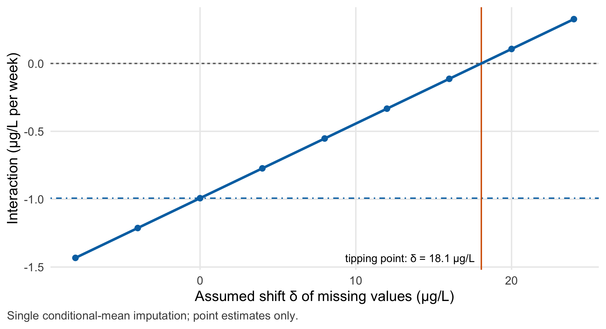
With weeks 0–4 only, the interaction is -1.45 µg/L per week (all visits: -0.99). The tipping point lies at δ = 18.1 µg/L (Figure 13.2), about 4.5 times the assumed measurement noise. Most filled visits belong to the complete-injury group (25 of 30), so optimistic assumptions about the people who left move this group’s slope upwards and the difference towards zero. Whether a shift of this size is plausible is a clinical judgement, not a statistical one. It should be made before the data are seen, by people who know why patients leave this kind of unit.
If the result stays unclear. When the tipping point lies within the range that clinicians find plausible, the honest summary is that the data do not settle the question. Report the MAR estimate, the tipping point and the reasons for leaving; do not search for the analysis that gives the desired answer. The next study can record reasons for missed visits, add a home or outpatient sample at week 8 and fix the sensitivity range in the analysis plan.
13.4 Counter-check
Change the dropout mechanism and keep everything else. Predict first: (1) If nobody drops out, will the three approaches agree? (2) Under MAR dropout, which approach is unbiased on average? (3) If leaving depends on the unmeasured current level and on the person’s own recovery rate (MNAR), in which direction will the mixed-model estimate move? Then run one hundred cohorts per mechanism. The simulation follows the logic of Monte Carlo experiments with explicit assumptions (see Strategy in R: law of large numbers and Monte Carlo).
set.seed(1300)
n_rep <- 100
n_singular <- 0                                   # singular fits are counted, not hidden
estimate_all <- function(obs) {
  per <- do.call(rbind, lapply(split(obs, obs$id), function(d)
    if (nrow(d) >= 2) data.frame(group = d$group[1], slope = coef(lm(selenium ~ week, data = d))[["week"]])))
  m <- suppressMessages(lmer(selenium ~ week * group + (week | id), data = obs, control = ctrl))
  if (isSingular(m)) n_singular <<- n_singular + 1
  c(pooled = coef(lm(selenium ~ week * group, data = obs))[["week:groupcomplete"]],
    per_person = diff(tapply(per$slope, per$group, mean))[[1]],
    mixed = fixef(m)[["week:groupcomplete"]])
}
replicates <- lapply(c(none = "none", mar = "mar", mnar = "mnar"), function(mech)
  t(replicate(n_rep, { d <- simulate_cohort(mech); estimate_all(d[d$observed, ]) })))
summary_rep <- do.call(rbind, lapply(names(replicates), function(mech) {
  r <- replicates[[mech]]
  data.frame(mechanism = mech, approach = colnames(r), mean = colMeans(r),
             mc_se = apply(r, 2, sd) / sqrt(n_rep))
}))
rownames(summary_rep) <- NULL
summary_rep$mean <- round(summary_rep$mean, 2); summary_rep$mc_se <- round(summary_rep$mc_se, 3)
summary_rep
#> mechanism approach mean mc_se
#> 1 none pooled -0.95 0.029
#> 2 none per_person -0.95 0.029
#> 3 none mixed -0.95 0.029
#> 4 mar pooled -0.81 0.044
#> 5 mar per_person -1.34 0.072
#> 6 mar mixed -1.02 0.036
#> 7 mnar pooled -0.83 0.035
#> 8 mnar per_person -0.93 0.071
#> 9 mnar mixed -0.89 0.032m_of <- function(mech, appr) summary_rep$mean[summary_rep$mechanism == mech & summary_rep$approach == appr]
stopifnot(
max(abs(replicates$none[, "pooled"] - replicates$none[, "mixed"])) < 1e-6, # complete data: identical
max(abs(replicates$none[, "per_person"] - replicates$none[, "mixed"])) < 1e-6,
abs(m_of("mar", "mixed") - (-1)) < 0.1, # MAR: mixed model unbiased within simulation error
m_of("mar", "pooled") > -0.9, # MAR: pooled estimate attenuated
m_of("mnar", "mixed") > m_of("mar", "mixed") # MNAR: mixed model moves towards zero
)The results answer the three predictions. With complete data, all three approaches give identical estimates in every cohort: in a balanced design, the mixed model’s fixed slope equals the pooled and the per-person slope. Under MAR dropout, the mixed model is unbiased on average (-1.02 against −1.00), the pooled regression is pulled towards zero (-0.81) and the per-person slopes are pushed away from it (-1.34), because people who leave after a low value contribute short, steep lines. Under MNAR, the mixed model also drifts towards zero (-0.89): it can only use what was observed. In 11 of 300 fits, the random-slope variance was estimated at the boundary; these fits are counted and kept. The lesson for the consultant’s question is that agreement between baseline and mixed model is reassuring only when few visits are missing. Disagreement is a signal to examine the reasons for leaving.
13.5 Consequences for patients and operations
Patients and ethics. The people who left were mostly from the complete-injury group, and they had low values. They are exactly the people a supplementation trial would target, and the estimate is least certain for them. A protocol should not rest on a slope that describes the people who managed to come back. Each extra blood draw is a burden for people with a new spinal cord injury; the next study should place samples where care already happens (ward rounds, rehabilitation visits) and record every reason for a missed visit. A group-level slope is a research finding, not an individual prognosis, and should not be communicated to patients as one (Chapter 21).
Data protection. A small cohort with a rare injury level, age, sex and exact visit dates can identify a person even without a name. The CSV file of this chapter is synthetic. With real data, share weeks since admission rather than dates, pseudonymised IDs and only the variables needed for the analysis; the questions of access and re-use are treated in Chapter 23 and Chapter 26.
Regulation and security. A slope used as a research end point does not make the analysis a medical device. The question would arise if software computed individual recovery forecasts from biomarker courses and clinicians used them to choose a treatment; Chapter 22 sets out how intended purpose drives that classification. Information security is indirectly relevant: the analysis data set, the code and the package versions must be versioned so that the numbers in the meeting can be reproduced (Chapter 4).
13.6 Look up and transfer
Reviewer question. How many persons, not measurements, contribute to the late part of each group’s course, and how far does the interaction move under a plausible MNAR scenario?
Self-test. A second synthetic cohort studies zinc after spinal cord injury. Here, people who recover well are discharged home after week 4 and their week-6 and week-8 values are missing; people who do poorly stay on the ward. In which direction is the pooled regression biased for the group with most discharges, and what would a sensitivity analysis need to assume?
TipAnswer
The late measurements now come from people with a poorer course, so the pooled slope of the group with most discharges is too flat. The mixed model under MAR corrects this only as far as the early values already reveal who is recovering well. If discharge depends on improvement that was not yet measured, the data are MNAR, and the mixed model is also too flat for that group. A sensitivity analysis would shift the missing late values upwards (positive δ) and report the δ at which the conclusion changes. Recording the reason “discharged home” makes the mechanism visible.
Annotated sources.
- Matthews et al. (1990) – the case for summary measures such as the slope per person; the source of the baseline.
- Laird and Ware (1982) – the random-effects model for longitudinal data that underlies the mixed model.
- Bates et al. (2015) – the implementation used in the lab, including the model syntax and estimation method.
- Rubin (1976) – the formal definition of missing at random and when the missing-data mechanism can be ignored.
- Diggle and Kenward (1994) – why informative dropout biases longitudinal analyses and how to model it.
- Little et al. (2012) – recommendations for preventing missing data and for sensitivity analyses in clinical studies.
- Seelig et al. (2020) – a published observational study of selenium and copper after spinal cord injury; it motivates the question only, no values are used.
13.7 Further reading
- Chapter 3 – how missing values and denominators arise in clinical data, before any model.
- Chapter 16 – how much a small sample can say, and how to state the remaining uncertainty.
- Methods in R: Random-Slope Models – model formulation, diagnostics and warning signs.
- Methods in R: Sensitivity Analyses in Clinical Trials – the wider family of sensitivity analyses for missing outcomes.
- CTTIR Course 2, Week 2, Session 3 – RCBD and repeated measures → mixed models – a step-by-step lab from repeated measures to mixed models.
- CTTIR Course 3, Week 2, Session 1 – MCAR, MAR, MNAR and Session 3 – Linear mixed models with lme4 – missing-data mechanisms and their consequences for longitudinal models.
- CTTIR Tutorials: Mixed-Effects Models – Introduction – a short refresher on random effects and shrinkage.