14 Cluster, gradient or artefact
R. Heller · Date: 2026-08-30 · Last changed: 2026-11-09
14.1 Case and decision
A fictitious trauma research group has six routine values from the first day after major trauma in 300 people: C-reactive protein, interleukin-6, lactate, leukocytes, platelets and body temperature. A colleague shows a two-dimensional map in which the patients form three islands. The proposal is to call them “hyperinflammatory”, “intermediate” and “quiet” subtypes, to name them in the manuscript and to stratify a planned trial by subtype. The group leader has to decide whether the word “subtype” goes into the manuscript and the trial protocol. The data in this chapter are synthetic and were generated, on purpose, from a single continuous severity gradient without any groups. The task is to find out which analysis would have revealed that – and what evidence would be needed before a subtype label may change what happens to a patient.
14.2 Core reading
What the table contains. One row per person, six columns with six units: mg/L, pg/mL, mmol/L, 109/L twice and °C. The independent unit is the person; n = 300. Any clustering method needs a distance between two people, and that distance depends on how the six columns are put on a common scale. Without scaling, platelets (standard deviation 59 × 109/L) and interleukin-6 (61 pg/mL) dominate, while lactate (0.8 mmol/L) and temperature (0.5 °C) hardly count. After standardisation to z-scores, each marker counts equally. After a log transformation of the skewed markers, the distances change again. Scaling is a modelling decision with clinical content, not a technical preliminary. In the lab, k-means on the original units agrees with the z-score solution only with an adjusted Rand index of 0.37 (1 means identical partitions, 0 chance agreement): changing the units reassigns a large share of the patients.
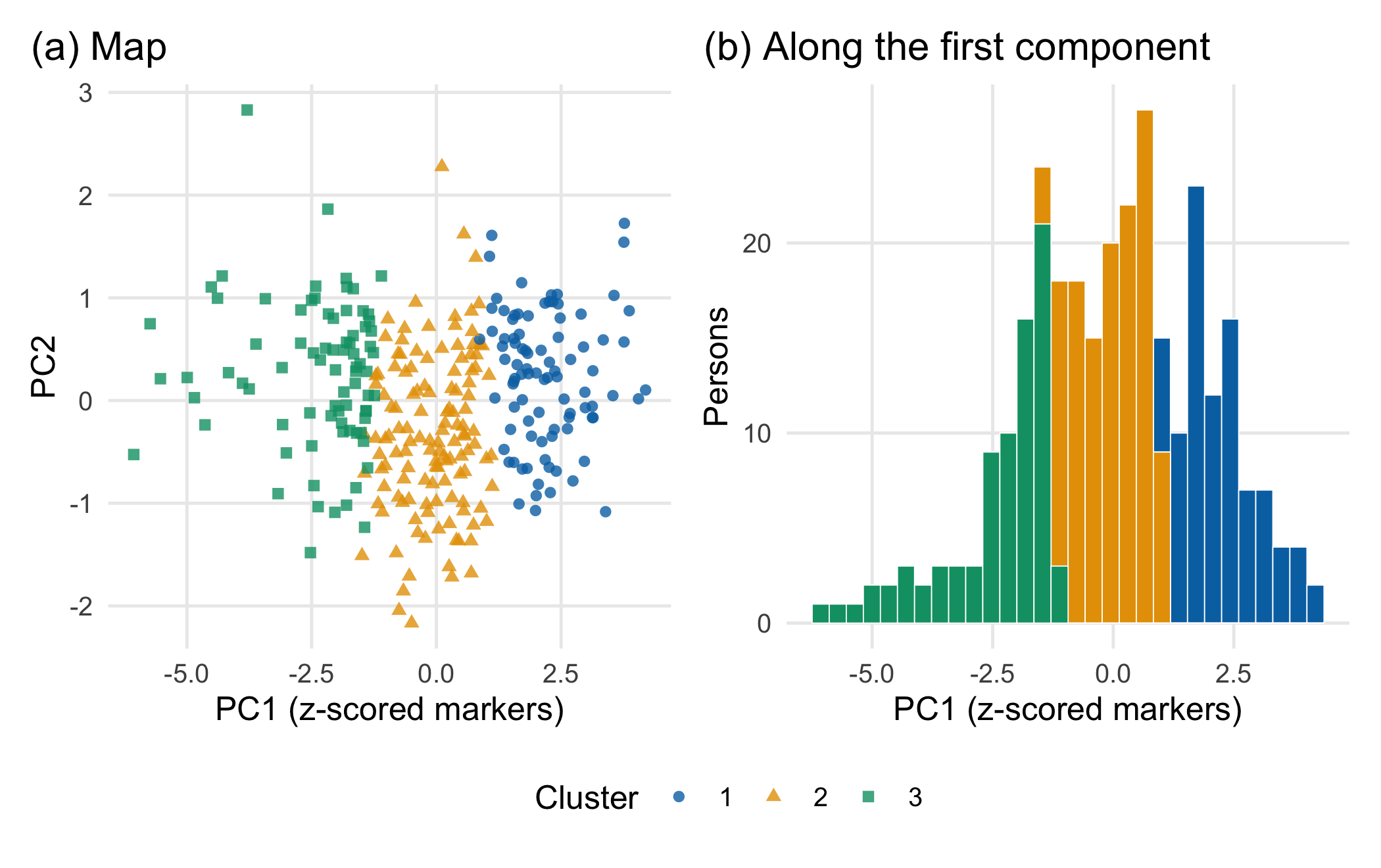
A gradient cut into slices. A principal component analysis (PCA) of the z-scores shows one dominant axis: the first component carries 62.5% of the variance and correlates at 0.93 with the hidden severity used to generate the data. k-means clustering with three clusters (Hartigan and Wong 1979) does what it is built to do: it minimises the sum of squared distances between each person and the nearest of three centres. On a gradient, it returns three slices (Figure 14.1). The left panel looks like three groups because the colours say so. The right panel shows the decisive detail: the cluster boundaries do not sit in empty regions. They cut through the densest part of the distribution.
Methods that agree for the wrong reason. Three further analyses seem to confirm the islands. A Gaussian mixture model (mclust, Scrucca et al. (2016)) selects 6 components by the Bayesian information criterion (BIC) on z-scores and 3 on log-transformed markers. BIC counts how many bell-shaped components are needed to describe the shape of the cloud; a skewed or curved cloud needs several, even without groups. Bootstrap stability looks reassuring as well: when the 300 persons are resampled and re-clustered a hundred times, the three clusters are recovered with mean Jaccard similarities between 0.77 and 0.91 (Hennig 2007). By the usual guidance for this measure, values above 0.75 count as stable (Hennig 2026). Stability, however, shows that the same cut is made each time, not that there is a seam to cut along. A knife set at the same place gives reproducible slices of a loaf.
The question behind the question. Every clustering algorithm returns as many groups as it is asked for. Asking “how many clusters are there?” therefore presupposes that there are clusters. The first question is a different one: is there any discontinuity in the population, or do the patients vary along one or a few continuous axes? Only if the answer is the former does the choice of k become meaningful.
What would distinguish groups from a gradient. A real group structure leaves a trough in the density between groups. A simple diagnostic compares the density of the first component at the boundary between two k-means clusters with the density at the two cluster centres. Here, the ratio is 1.18: the boundary lies where people are more frequent than at the centres. The counter-check (Section 14.4) builds a data set with a real gap and shows how this ratio falls.
UMAP islands. Two-dimensional maps such as UMAP (McInnes et al. 2018) are built to keep each person’s nearest neighbours close. The documentation of the reference implementation states that UMAP, like t-SNE, does not completely preserve density and can create false tears in clusters, yielding a finer clustering than is present in the data (McInnes 2026). Island sizes, gaps and distances between islands are not measurements; Chari and Pachter (2023) show how strongly such maps can distort the structure of single-cell data. A map is a reason to look, not evidence of subtypes.
The baseline. The biometrically sensible baseline for a gradient is a continuous score, here the first principal component. In the lab, a model for a synthetic day-7 organ dysfunction outcome fits better with the continuous score (AIC 326.0) than with the three cluster labels (AIC 337.1). Cutting the gradient into slices throws information away. A label also hides similarity: two patients who lie just either side of a boundary receive different names, while two patients at opposite ends of the same slice share one.
The most important assumption. A cluster label claims a discontinuity in the population. It is supported only if a gap survives changes of scaling, algorithm and sample, reappears in an independent cohort and the label adds information beyond a continuous score. Without this, “three subtypes” describes the analysis, not the patients.
Question for the workshop. Which observation would convince you that the three islands are subtypes rather than slices: the same islands after log transformation, a trough in the density, reproduction in another centre or a different treatment effect in a randomised trial? Rank the four and justify the order.
14.3 Lab
The lab needs mclust, cluster, ggplot2 and patchwork and runs in a few seconds.
14.3.1 Step 1: simulate a gradient without groups
All values are synthetic assumptions. A single latent severity score drives all six markers; three of them are right-skewed, as many inflammatory markers are. The day-7 outcome depends on the same score, continuously.
set.seed(1414)                                    # same data each time this chunk runs
n <- 300
make_markers <- function(severity) {              # one latent score drives all six markers
  m <- length(severity)
  data.frame(
    crp_mg_l          = pmax(1, 60 + 35 * severity + rnorm(m, 0, 20)),
    il6_pg_ml         = exp(3.6 + 0.8 * severity + rnorm(m, 0, 0.45)),
    lactate_mmol_l    = exp(log(1.8) + 0.30 * severity + rnorm(m, 0, 0.25)),
    leukocytes_10e9_l = pmax(1, 11 + 2.5 * severity + rnorm(m, 0, 2.5)),
    platelets_10e9_l  = pmax(20, 220 - 35 * severity + rnorm(m, 0, 45)),
    temperature_c     = 37.4 + 0.4 * severity + rnorm(m, 0, 0.35))
}
severity <- rnorm(n)                              # continuous, unimodal: no subtypes by construction
markers <- make_markers(severity)
organ_dysfunction <- rbinom(n, 1, plogis(-1.2 + 1.3 * severity))   # synthetic day-7 outcome
round(sapply(markers, function(x) c(median = median(x), sd = sd(x))), 2)
#> crp_mg_l il6_pg_ml lactate_mmol_l leukocytes_10e9_l platelets_10e9_l
#> median 62.95 38.73 1.81 10.94 213.73
#> sd 39.66 61.02 0.84 3.56 59.02
#> temperature_c
#> median 37.46
#> sd 0.5314.3.2 Step 2: three scalings and a PCA
log_vars <- c("crp_mg_l", "il6_pg_ml", "lactate_mmol_l")
x_raw <- as.matrix(markers)                       # original units
x_z <- scale(markers)                             # z-scores: every marker counts equally
markers_log <- markers
markers_log[log_vars] <- lapply(markers_log[log_vars], log)
x_logz <- scale(markers_log)                      # log for skewed markers, then z-scores
pca <- prcomp(x_z)
pc1_share <- summary(pca)$importance["Proportion of Variance", "PC1"]
cor_pc1 <- cor(pca$x[, 1], severity)
round(summary(pca)$importance[, 1:3], 3)
#> PC1 PC2 PC3
#> Standard deviation 1.936 0.773 0.702
#> Proportion of Variance 0.625 0.100 0.082
#> Cumulative Proportion 0.625 0.724 0.80614.3.3 Step 3: k-means with two to five clusters
The mean silhouette width compares, for every person, the distance to the own cluster with the distance to the nearest other cluster (Rousseeuw 1987); values near 1 indicate well-separated clusters.
library(cluster)
library(mclust)
set.seed(14141)
d_z <- dist(x_z)
km <- lapply(2:5, function(k) kmeans(x_z, centers = k, nstart = 25))
silhouette_mean <- sapply(km, function(m) mean(silhouette(m$cluster, d_z)[, "sil_width"]))
names(silhouette_mean) <- paste0("k=", 2:5)
cluster_ref <- km[[2]]$cluster                    # reference solution: z-scores, k = 3
cluster_raw <- kmeans(x_raw, centers = 3, nstart = 25)$cluster
cluster_log <- kmeans(x_logz, centers = 3, nstart = 25)$cluster
ari_raw <- adjustedRandIndex(cluster_ref, cluster_raw)   # 1 = identical partition, 0 = chance agreement
ari_log <- adjustedRandIndex(cluster_ref, cluster_log)
round(c(silhouette_mean, ARI_raw_vs_z = ari_raw, ARI_log_vs_z = ari_log), 3)
#> k=2 k=3 k=4 k=5 ARI_raw_vs_z ARI_log_vs_z
#> 0.335 0.247 0.233 0.192 0.368 0.464The adjusted Rand index (ARI) compares two partitions of the same people and is 0 for chance agreement (Hubert and Arabie 1985). Changing only the scaling reassigns a large share of the patients.
14.3.4 Step 4: a Gaussian mixture model
mc_z <- Mclust(x_z, G = 1:6, verbose = FALSE)
mc_log <- Mclust(x_logz, G = 1:6, verbose = FALSE)
c(z_scores = mc_z$G, log_z = mc_log$G)
#> z_scores log_z
#> 6 3c(model_z = mc_z$modelName, model_log = mc_log$modelName)#> model_z model_log
#> "VVI" "EEE"14.3.5 Step 5: bootstrap stability
For each resample, the persons are drawn with replacement, k-means is rerun, and every original cluster is compared with its best-matching new cluster on the persons present in both (Jaccard similarity: shared persons divided by persons in either). This follows the logic of Hennig’s cluster-wise stability assessment; the same procedure is available as fpc::clusterboot() (Hennig 2007, 2026).
bootstrap_stability <- function(x, k, n_boot = 100) {
  ref <- kmeans(x, centers = k, nstart = 25)$cluster
  jac <- matrix(NA_real_, n_boot, k)
  ari <- numeric(n_boot)
  for (b in seq_len(n_boot)) {
    idx <- sample(nrow(x), replace = TRUE)
    new <- kmeans(x[idx, ], centers = k, nstart = 10)$cluster
    present <- unique(idx)
    new_present <- new[match(present, idx)]       # new cluster of each person in the resample
    for (j in seq_len(k)) {
      a <- present[ref[present] == j]
      jac[b, j] <- max(sapply(seq_len(k), function(m) {
        bset <- present[new_present == m]
        length(intersect(a, bset)) / length(union(a, bset))
      }))
    }
    ari[b] <- adjustedRandIndex(ref[present], new_present)
  }
  list(jaccard = colMeans(jac), ari_median = median(ari))
}
set.seed(14142)
stab <- lapply(2:4, function(k) bootstrap_stability(x_z, k))
jac <- list(k2 = stab[[1]]$jaccard, k3 = stab[[2]]$jaccard, k4 = stab[[3]]$jaccard)
lapply(jac, round, 2)
#> $k2
#> [1] 0.95 0.94
#>
#> $k3
#> [1] 0.82 0.91 0.77
#>
#> $k4
#> [1] 0.89 0.96 0.84 0.7214.3.6 Step 6: look for a trough instead of a cluster count
valley_ratio_of <- function(x) {
  pc <- prcomp(x)$x[, 1]
  cl <- kmeans(x, centers = 2, nstart = 25)$cluster
  centres <- tapply(pc, cl, mean)
  dens <- density(pc, bw = "SJ")                  # kernel density of the first component
  f <- approxfun(dens$x, dens$y)
  f(mean(centres)) / mean(f(centres))             # density at the boundary / density at the centres
}
set.seed(14143)
valley_ratio <- valley_ratio_of(x_z)
round(valley_ratio, 2)
#> [1] 1.18A ratio well below 1 points to a trough between two groups; a ratio near or above 1 means that the boundary runs through a dense region. The ratio is a didactic diagnostic, not a formal test, and it looks only along the first component.
14.3.7 Step 7: the continuous baseline
fit_cluster <- glm(organ_dysfunction ~ factor(cluster_ref), family = binomial)
fit_score <- glm(organ_dysfunction ~ pca$x[, 1], family = binomial)
aic_cluster <- AIC(fit_cluster)
aic_pc1 <- AIC(fit_score)
c(AIC_three_clusters = round(aic_cluster, 1), AIC_continuous_score = round(aic_pc1, 1))
#> AIC_three_clusters AIC_continuous_score
#> 337.1 326.014.3.8 Step 8: collect the variants and check the target values
variants <- data.frame(
  Variant = c("z-scores, k-means, k = 2", "z-scores, k-means, k = 3 (reference)", "z-scores, k-means, k = 4",
              "original units, k-means, k = 3", "log + z-scores, k-means, k = 3",
              "z-scores, Gaussian mixture (BIC)", "log + z-scores, Gaussian mixture (BIC)"),
  Silhouette = c(cdsr_number(silhouette_mean[1:3], 2), "", "", "", ""),
  Jaccard = c(cdsr_number(sapply(jac, min), 2), "", "", "", ""),
  ARI = c("", "1.00", "", cdsr_number(ari_raw, 2), cdsr_number(ari_log, 2), "", ""),
  Components = c("2", "3", "4", "3", "3", as.character(mc_z$G), as.character(mc_log$G)))
knitr::kable(variants, align = "lrrrr")| Variant | Silhouette | Jaccard | ARI | Components |
|---|---|---|---|---|
| z-scores, k-means, k = 2 | 0.34 | 0.94 | 2 | |
| z-scores, k-means, k = 3 (reference) | 0.25 | 0.77 | 1.00 | 3 |
| z-scores, k-means, k = 4 | 0.23 | 0.72 | 4 | |
| original units, k-means, k = 3 | 0.37 | 3 | ||
| log + z-scores, k-means, k = 3 | 0.46 | 3 | ||
| z-scores, Gaussian mixture (BIC) | 6 | |||
| log + z-scores, Gaussian mixture (BIC) | 3 |
stopifnot(
  pc1_share > 0.5, abs(cor_pc1) > 0.9,            # one dominant axis that tracks the hidden gradient
  mc_z$G > 1, mc_log$G > 1,                       # BIC prefers several components although there is no group
  min(jac$k3) > 0.75,                             # "stable" by the usual guidance ...
  valley_ratio > 0.8,                             # ... but no trough at the boundary
  ari_raw < 0.6,                                  # scaling changes the partition substantially
  aic_pc1 < aic_cluster                           # the continuous score is the better baseline
)
14.3.9 Step 9: an external test plan
A subtype hypothesis becomes testable when the analysis is frozen before new data are seen. Table 14.2 lists a minimal plan; each line names what would count against the hypothesis.
| Element | Fixed in advance | Counts against the subtype hypothesis |
|---|---|---|
| Pipeline | markers, units, transformation, scaling, algorithm, k, seed, centres | any change after seeing the new cohort |
| Cohort | another centre or period, same assays and units, consecutive patients | selected or differently measured cohort |
| Reproduction | assign new patients to the frozen centres; recluster independently; compare (ARI, prediction strength (Tibshirani and Walther 2005)) | low agreement between frozen and new partition |
| Discontinuity | trough between clusters along the main axis | boundary in a dense region (ratio near or above 1) |
| Added value | clusters versus continuous score for a pre-specified outcome | no gain over the continuous score |
| Consequence | differential treatment effect in randomised data | effect identical across clusters |
The last line is what the trial stratification would need. A published example of the kind of evidence it requires is the latent class analysis of two randomised trials in acute respiratory distress syndrome, in which two subphenotypes were found in both cohorts and the effect of the ventilation strategy differed by subphenotype in a secondary analysis (Calfee et al. 2014). Even there, the authors framed the result as useful for selecting patients for future trials, not as a basis for treatment choice.
NoteOther implementation: Python/umap-learn
The reference implementation of UMAP is the Python package umap-learn (version 0.5.12, April 2026; documentation) (McInnes et al. 2018). Its concrete advantage is direct access to the original algorithm and its parameters (n_neighbors, min_dist, metric), which matters when a published map is to be reproduced. For a fair comparison with an R workflow, the input matrix (same persons, same transformation and scaling), the parameters, the random seed and the number of dimensions must be identical; even then, different random initialisations can move islands. Status: conceptual comparison, not run. Any cluster seen on such a map must pass the same checks as above on the original, unprojected data.
If the result stays unclear. “No evidence for discrete subtypes; the markers vary along one continuous axis” is a finding worth reporting. It comes with the continuous score, its distribution and the outcome model, which others can test. When some diagnostics support groups and others do not, report all of them and keep the language at “candidate clusters” until the external plan has been run.
14.4 Counter-check
Change the data, not the method: generate the same six markers from a severity score with a real gap – two groups of 150 people centred at −1.2 and +1.2 with a within-group spread of 0.45 (assumption). Predict first: which of the diagnostics will change markedly – the BIC component count, the bootstrap Jaccard similarity, the silhouette width or the trough ratio?
set.seed(1415)
severity_gap <- c(rnorm(n / 2, -1.2, 0.45), rnorm(n / 2, 1.2, 0.45))
x_gap <- scale(make_markers(severity_gap))
km_gap <- kmeans(x_gap, centers = 2, nstart = 25)
km_grad2 <- km[[1]]
compare <- data.frame(
  Diagnostic = c("mean silhouette, k = 2", "smallest bootstrap Jaccard, k = 2", "trough ratio",
                 "Gaussian mixture components (BIC)"),
  Gradient = c(silhouette_mean[["k=2"]], min(jac$k2), valley_ratio, mc_z$G),
  Gap = c(mean(silhouette(km_gap$cluster, dist(x_gap))[, "sil_width"]),
          min(bootstrap_stability(x_gap, 2)$jaccard),
          valley_ratio_of(x_gap),
          Mclust(x_gap, G = 1:6, verbose = FALSE)$G))
compare$Gradient <- round(compare$Gradient, 2); compare$Gap <- round(compare$Gap, 2)
compare
#> Diagnostic Gradient Gap
#> 1 mean silhouette, k = 2 0.34 0.49
#> 2 smallest bootstrap Jaccard, k = 2 0.94 0.99
#> 3 trough ratio 1.18 0.35
#> 4 Gaussian mixture components (BIC) 6.00 4.00stopifnot(compare$Gap[3] < 0.5, compare$Gradient[3] > 0.8, # the trough separates the two situations
compare$Gap[1] > compare$Gradient[1], # silhouette rises, but modestly
abs(compare$Gap[2] - compare$Gradient[2]) < 0.1) # stability hardly differsboundary_of <- function(x, cl) mean(tapply(prcomp(x)$x[, 1], cl, mean))
hist_df <- rbind(data.frame(scenario = "Gradient (no groups)", pc1 = prcomp(x_z)$x[, 1]),
data.frame(scenario = "Two groups with a gap", pc1 = prcomp(x_gap)$x[, 1]))
bounds <- data.frame(scenario = c("Gradient (no groups)", "Two groups with a gap"),
b = c(boundary_of(x_z, km_grad2$cluster), boundary_of(x_gap, km_gap$cluster)))
ggplot(hist_df, aes(pc1)) +
geom_histogram(bins = 30, fill = cdsr_colours[["skyblue"]], colour = "white", linewidth = 0.2) +
geom_vline(data = bounds, aes(xintercept = b), colour = cdsr_colours[["red"]], linetype = cdsr_linetypes[[2]]) +
facet_wrap(~ scenario) +
labs(x = "PC1 (z-scored markers)", y = "Persons") +
theme_cdsr()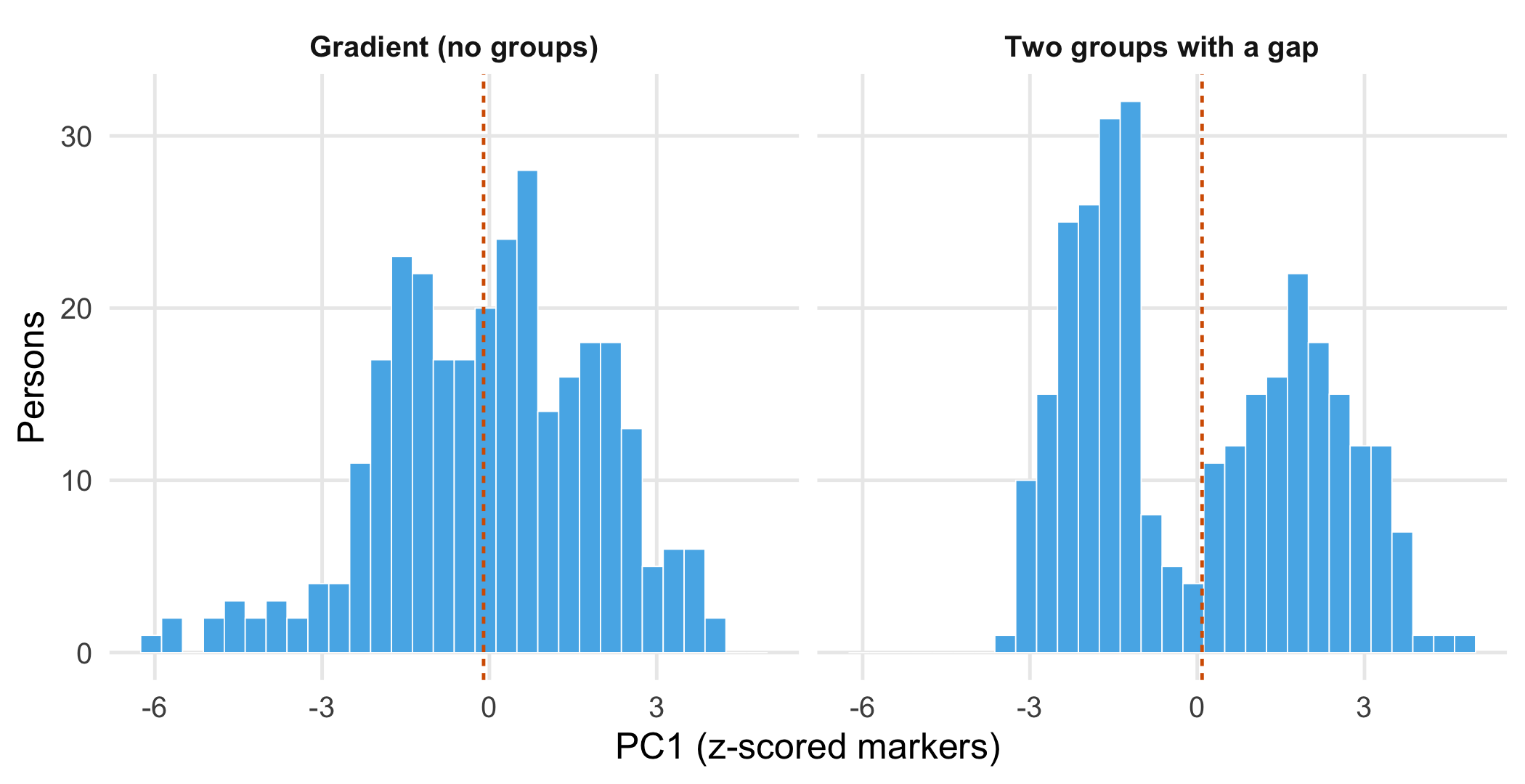
The trough ratio falls from 1.18 to 0.35, and the silhouette width rises from 0.34 to 0.49. Bootstrap stability hardly changes (0.94 versus 0.99): it was already high for the gradient. The mixture model selects 4 components for two groups, which again shows that the BIC count describes the shape of the density, not the number of patient groups. Only the diagnostics that look for empty space between groups separate the two situations.
14.5 Consequences for patients and operations
Patients and ethics. A subtype label travels. It enters records, referral letters and conversations, and it can change expectations about recovery. A person labelled “hyperinflammatory” because their values lie just across an arbitrary boundary may receive a different treatment from a neighbour with almost identical values. A subtype name therefore needs a justified consequence: a treatment, monitoring or prognosis decision that differs by subtype and has been shown to do so, as in the external plan above. Without it, the continuous score is more honest and loses less information. If the markers differ systematically by sex, age or laboratory method, clusters can become proxies for these characteristics; check the distribution of such variables across clusters before naming them (Chapter 21).
Regulation. Exploratory clustering in a research data set is not a medical device. If software assigned patients to subtypes in order to select a treatment, its intended purpose would have to be assessed under the medical device rules (Chapter 22).
Data protection and security. A cluster label derived from personal data is itself personal data. Small clusters with unusual marker combinations can make individuals recognisable in published figures or supplementary tables (Chapter 23). Security is only indirectly relevant: the frozen pipeline of the external plan, including centres and seed, must be stored and versioned so that the test cannot be adjusted after the fact.
14.6 Look up and transfer
Reviewer question. Did the authors show a gap between clusters that survives a change of scaling and reappears in an independent cohort, and does the cluster label predict the outcome better than a continuous score?
Self-test. A manuscript reports four “immune subtypes” after polytrauma, found with k-means on z-scored markers. The authors cite mean bootstrap Jaccard similarities above 0.85 and a BIC-selected mixture model with four components as validation. What is missing?
TipAnswer
Both arguments are compatible with a continuous gradient: k-means cuts a gradient reproducibly, and BIC adds components to describe a skewed or curved density. Missing are evidence of a discontinuity (a trough or clear separation that survives other scalings and algorithms), reproduction in an independent cohort with a frozen pipeline, and a comparison with a continuous score. A treatment consequence would additionally need a differential effect in randomised data.
Annotated sources.
- Hennig (2007) – cluster-wise bootstrap stability with the Jaccard similarity; the method behind Step 5.
- Hennig (2026) – documentation of
clusterboot(), including the usual interpretation thresholds for the mean Jaccard similarity. - Scrucca et al. (2016) – the Gaussian mixture models and BIC-based model choice used in Step 4.
- Hartigan and Wong (1979) – the k-means algorithm that R’s
kmeans()uses by default. - Rousseeuw (1987) and Hubert and Arabie (1985) – silhouette width and adjusted Rand index.
- Tibshirani and Walther (2005) – prediction strength as a check of whether clusters reproduce in new data.
- McInnes et al. (2018), McInnes (2026) and Chari and Pachter (2023) – how UMAP works, the warning about false tears, and how far two-dimensional embeddings can distort structure.
- Calfee et al. (2014) – a published subphenotype analysis that tested reproduction in two cohorts and a differential treatment effect.
14.7 Further reading
- Chapter 12 – phenotypes from segmented tissue images, where cluster boundaries also depend on upstream choices.
- Chapter 19 – how to plan the external cohort that the test plan needs.
- Methods in R: Gaussian Mixture Models and k-Means Clustering – assumptions, diagnostics and warning signs of both methods.
- Methods in R: UMAP and t-SNE – Overview – what two-dimensional embeddings preserve and what they do not.
- Methods in R: Centring and Scaling Predictors – why the scale of a variable changes its weight.
- CTTIR Course 4, Week 1, Session 4 – Clustering: k-means, hierarchical, model-based and Session 5 – UMAP and t-SNE – hands-on labs with the same methods.
- CTTIR Tutorials: Cluster Validation – Silhouette – interpreting silhouette widths.