2 Describe, predict, explain
R. Heller · Date: 2025-03-09 · Last changed: 2026-11-09
2.1 Case and decision
A geriatric trauma team reviews its results after hip fracture surgery. The in-house standard aims to operate within 24 hours of admission (an assumption of this case, not a guideline statement). A colleague presents an analysis of the intensive care database. Among older patients with hip fracture who needed intensive care, those whose surgery was delayed beyond 24 hours were less often unable to walk independently at day 90. Someone suggests that the push for early surgery could be relaxed for complex patients. The head of department has to decide whether to change the standard. Before looking at any model, the team needs to know which question the analysis answered, and whether it is the question the decision requires.
2.2 Core reading
2.2.1 Three questions about the same variables
The same variables can serve three different purposes. Hernán and colleagues call them description, prediction and counterfactual prediction, the last being the task of causal inference (Hernán et al. 2019). Shmueli showed that a model built to explain is judged by different criteria from a model built to predict, even if the software call looks the same (Shmueli 2010). Table 2.1 applies this to the case.
| Describe | Predict | Explain (causal) | |
|---|---|---|---|
| Example | What proportion of patients aged 70 or over with hip fracture could not walk independently at day 90, by timing of surgery? | For a patient like Ms K., what is the probability at admission of not walking independently at day 90? | How would the proportion not walking at day 90 change if all patients were operated within 24 hours rather than later? |
| Time zero | Admission | Moment of prediction (here: admission) | Moment of the decision on timing (admission) |
| Target quantity | Proportions with their denominators | An individual risk; judged by accuracy and calibration | A risk difference between two hypothetical strategies |
| ‘Surgery delayed’ | Grouping variable | Predictor, if known at the moment of prediction | The intervention |
| ‘ICU admission’ | Defines a subgroup and changes the population | Not yet known at admission; a valid predictor only for a later time zero | A consequence of the intervention; must not be selected or adjusted for |
A descriptive answer is correct if the counts are right and the denominators are named. A prognostic answer is useful if its predictions are accurate in the population where they will be used. A causal answer requires something more: an assumption about how the variables influence each other.
2.2.2 The target quantity has to be written down
For the causal question, the target quantity, the estimand, has to be specified before the analysis. The ICH E9(R1) addendum lists its attributes: the treatment conditions to be compared, the population, the variable measured in each patient, the handling of intercurrent events (events after the start of treatment, such as death or transfer, that affect the measurement or its meaning) and the population-level summary (International Council for Harmonisation 2019). For the case: older patients admitted with hip fracture; surgery within 24 hours versus later; not walking independently at day 90; death before day 90 counted as not walking (a composite strategy, one of several possible choices); the difference in proportions. Hernán and Robins recommend describing the randomised trial one would ideally run, the target trial, and then aligning eligibility, assignment and time zero in the observational data with it (Hernán and Robins 2016). In such a trial, nobody would be enrolled only after reaching the intensive care unit.
2.2.3 A small causal diagram
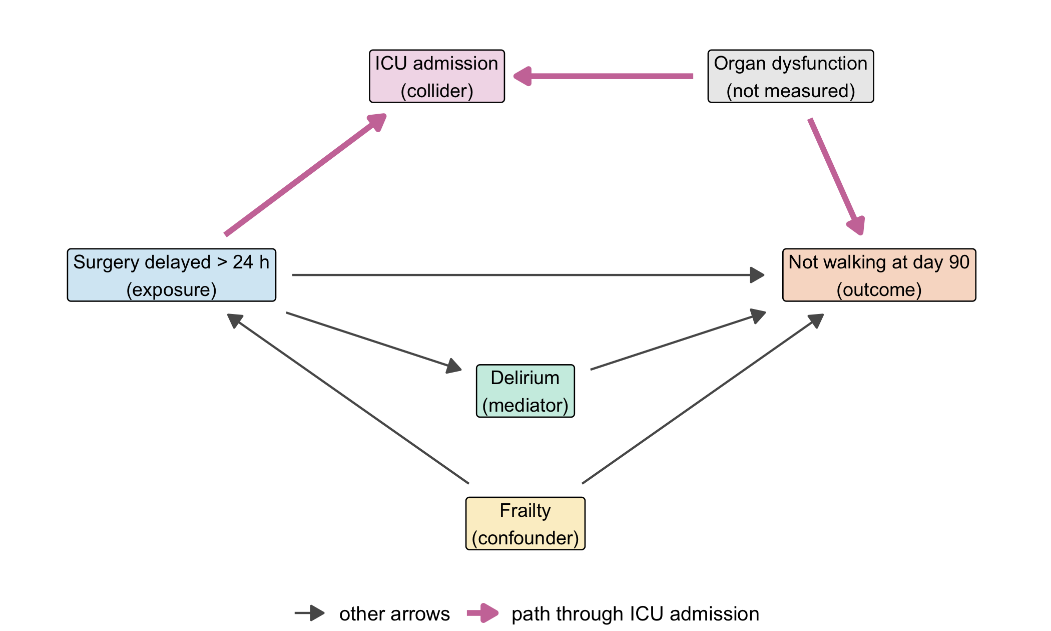
Figure 2.1 draws the assumptions as a directed acyclic graph (DAG). Each arrow means “may directly influence”; a missing arrow is a strong claim that there is no direct influence.
Three roles matter. Frailty is a confounder: it makes delay more likely (frail patients often need medical optimisation first) and independently worsens walking. Comparing delayed with early surgery without accounting for frailty mixes the two. Delirium is a mediator: it lies on a path from delay to walking. For the total effect of delay, one does not adjust for it, because that would remove part of the effect we want to estimate. ICU admission is a collider on the path delay → ICU ← organ dysfunction → walking: two arrows collide in it. That path is closed as long as we leave ICU admission alone. Selecting only ICU patients, or adjusting for ICU admission, opens it (Hernán et al. 2004). The R package dagitty reads such a graph and lists the variables that are sufficient for adjustment (Textor et al. 2016); here the answer is frailty alone.
2.2.4 Why the sign flips
In the Lab we simulate 4,000 patients whose data follow exactly this graph. The true effect of delay is built in: 7.5 percentage points more patients not walking at day 90 (assumption). In the whole cohort, after adjusting for frailty, the estimate is +7.2 points. Among the 767 ICU patients alone it is −9.9 points: delay seems protective (both synthetic).
The explanation lies in why patients reach the ICU. Patients operated early usually got there because of organ dysfunction; in the simulation this applies to 81% of them. Patients with delayed surgery often got there because of complications of the waiting time, and only 40% had organ dysfunction. Organ dysfunction strongly impairs recovery. Within the ICU, the early-surgery group is therefore sicker, and delay looks favourable. The same mechanism has been described for studies that sampled only hospitalised or tested patients during the COVID-19 pandemic (Griffith et al. 2020).
2.2.5 What would answer the head of department
The ICU analysis is not useless; it correctly describes patients who reached intensive care. It cannot answer the question on the table, because the decision about timing is taken at admission and applies to all admitted patients. An analysis that could inform the standard starts at admission (time zero), includes every older patient admitted with hip fracture, compares surgery within 24 hours with later surgery, adjusts for the confounders named in the graph (here frailty), treats death before day 90 according to the estimand, and does not select or adjust on anything that happens after the timing decision, including ICU admission and delirium. If organ dysfunction at admission were recorded, it would be measured before the decision and could be used as well; recorded after the decision, it would be a consequence. The whole difference lies in the order of events, which is why time zero comes first.
The DAG is an assumption, not a result. The data alone cannot show whether delay causes ICU admission; clinical knowledge has to justify that arrow, and with it the decision not to analyse ICU patients separately.
Question for the workshop: Which of the three questions does the head of department need answered? Write down its time zero, its population and the one variable you would refuse to select on — and say why.
2.3 Lab
2.3.1 Step 1: the graph as an R object
The DAG in Figure 2.1 was defined with the following code (the drawing part is ordinary ggplot2).
library(ggplot2)
library(dagitty)

dag_b02 <- dagitty('dag {
  delay    [exposure, pos="0,0"]
  walk     [outcome,  pos="4,0"]
  frailty  [pos="2,1.5"]
  delirium [pos="2,0.7"]
  icu      [pos="1.5,-1.2"]
  organ    [latent, pos="3.5,-1.2"]
  frailty -> delay
  frailty -> walk
  delay -> walk
  delay -> delirium -> walk
  delay -> icu
  organ -> icu
  organ -> walk
}')

# node positions (dagitty counts y downwards, so the sign is flipped for plotting)
pos   <- coordinates(dag_b02)
nodes <- data.frame(name = names(pos$x), x = pos$x, y = -pos$y)
labels <- c(delay = "Surgery delayed > 24 h\n(exposure)", walk = "Not walking at day 90\n(outcome)",
            frailty = "Frailty\n(confounder)", delirium = "Delirium\n(mediator)",
            icu = "ICU admission\n(collider)", organ = "Organ dysfunction\n(not measured)")
nodes$label <- labels[nodes$name]

# arrows run from box edge to box edge; box half-width grows with the longest label line
longest  <- sapply(strsplit(nodes$label, "\n"), function(l) max(nchar(l)))
nodes$hw <- 0.026 * longest + 0.06          # half-width in plot units
hh <- 0.21                                  # half-height in plot units
e <- as.data.frame(edges(dag_b02))[, c("v", "w")]
from <- nodes[match(e$v, nodes$name), ]
to   <- nodes[match(e$w, nodes$name), ]
dx <- to$x - from$x; dy <- to$y - from$y; len <- sqrt(dx^2 + dy^2)
ux <- dx / len; uy <- dy / len
gap_from <- pmin(from$hw / abs(ux), hh / abs(uy)) + 0.05
gap_to   <- pmin(to$hw / abs(ux), hh / abs(uy)) + 0.05
arrows_df <- data.frame(x = from$x + gap_from * ux, y = from$y + gap_from * uy,
                        xend = to$x - gap_to * ux, yend = to$y - gap_to * uy,
                        path = ifelse(e$v == "organ" | e$w == "icu",
                                      "path through ICU admission", "other arrows"))

ggplot() +
  geom_segment(data = arrows_df,
               aes(x = x, y = y, xend = xend, yend = yend, colour = path, linewidth = path),
               arrow = arrow(length = unit(2.4, "mm"), type = "closed")) +
  geom_label(data = nodes, aes(x = x, y = y, label = label), size = 3.2, linewidth = 0.3,
             fill = c(delay = "#D6E9F5", walk = "#F8DCCB", frailty = "#FBEFCC", delirium = "#CCEDE3",
                      icu = "#F2DCE9", organ = "grey92")[nodes$name]) +
  scale_colour_manual(values = c("other arrows" = "grey35",
                                 "path through ICU admission" = cdsr_colours[["purple"]]), name = NULL) +
  scale_linewidth_manual(values = c("other arrows" = 0.5, "path through ICU admission" = 1.3), name = NULL) +
  coord_cartesian(xlim = c(-0.7, 4.7), ylim = c(-1.7, 1.5)) +
  theme_void(base_size = 12) + theme(legend.position = "bottom")
dagitty can now answer questions about the graph. adjustmentSets() lists the minimal sets of variables that block every non-causal path between exposure and outcome; isAdjustmentSet() tests a proposed set.
adjustmentSets(dag_b02, effect = "total")#> { frailty }checks <- c(
frailty = isAdjustmentSet(dag_b02, "frailty"),
frailty_and_icu = isAdjustmentSet(dag_b02, c("frailty", "icu")),
frailty_and_delirium = isAdjustmentSet(dag_b02, c("frailty", "delirium"))
)
checks#> frailty frailty_and_icu frailty_and_delirium
#> TRUE FALSE FALSEstopifnot(identical(unname(checks), c(TRUE, FALSE, FALSE)))Adding ICU admission breaks the adjustment because it opens the collider path. Adding delirium breaks it for the total effect because it blocks part of the effect itself. paths() shows which paths are open after selecting on ICU admission:
paths(dag_b02, Z = c("frailty", "icu"))#> $paths
#> [1] "delay -> delirium -> walk" "delay -> icu <- organ -> walk"
#> [3] "delay -> walk" "delay <- frailty -> walk"
#>
#> $open
#> [1] TRUE TRUE TRUE FALSEThe path delay -> icu <- organ -> walk is listed as open (TRUE). The back-door path through frailty is closed.
2.3.2 Step 2: data that follow the graph
The function below simulates patients exactly as the graph says. Every number in it is a teaching assumption. Each line draws one variable with rbinom(), which returns 1 (yes) with the stated probability and 0 (no) otherwise. The seed inside the function makes the result identical on every computer.
simulate_cohort <- function(n = 4000, delay_to_icu = 0.25, seed = 2402) {
  set.seed(seed)
  frailty  <- rbinom(n, 1, 0.40)                                   # 40% frail
  organ    <- rbinom(n, 1, 0.20)                                   # 20% acute organ dysfunction
  delay    <- rbinom(n, 1, 0.25 + 0.20 * frailty)                  # frailty -> delay
  delirium <- rbinom(n, 1, 0.15 + 0.15 * delay)                    # delay -> delirium
  icu      <- rbinom(n, 1, 0.03 + delay_to_icu * delay + 0.45 * organ)   # delay, organ -> ICU
  not_walk <- rbinom(n, 1, 0.10 + 0.06 * delay + 0.10 * delirium + 0.15 * frailty + 0.35 * organ)
  data.frame(frailty, organ, delay, delirium, icu, not_walk)
}
cohort <- simulate_cohort()
true_effect <- 0.06 + 0.10 * 0.15          # direct part + part through delirium
c(patients = nrow(cohort), icu = sum(cohort$icu), true_effect = true_effect)
#> patients icu true_effect
#> 4000.000 767.000 0.075The true total effect is 0.06 (direct) plus 0.10 × 0.15 (the extra delirium caused by delay, times the harm of delirium) = 0.075, i.e. 7.5 percentage points.
2.3.3 Step 3: three analyses, three answers
A linear model with a 0/1 outcome, lm(not_walk ~ delay + frailty), returns the risk difference for delay directly as its coefficient. This is enough for a simulation in which all effects add up; it is not a general recommendation for binary outcomes (Methods in R: Multiple Linear Regression explains the model).
risk_diff <- function(formula, data) coef(lm(formula, data = data))[["delay"]]
estimates <- c(
  describe_all          = risk_diff(not_walk ~ delay, cohort),
  adjust_frailty        = risk_diff(not_walk ~ delay + frailty, cohort),
  adjust_frailty_delir  = risk_diff(not_walk ~ delay + frailty + delirium, cohort),
  icu_only              = risk_diff(not_walk ~ delay + frailty, cohort[cohort$icu == 1, ])
)
round(100 * estimates, 1)   # percentage points
#> describe_all adjust_frailty adjust_frailty_delir
#> 10.4 7.2 5.8
#> icu_only
#> -9.9stopifnot(round(100 * estimates[["adjust_frailty"]], 1) == 7.2,
round(100 * estimates[["icu_only"]], 1) == -9.9,
sum(cohort$icu) == 767)The crude difference (+10.4 points) is a correct description of this cohort but overstates the effect, because frail patients are delayed more often. Adjusting for frailty gives +7.2 points, close to the built-in 7.5. Adding delirium gives +5.8 points: roughly the direct part only. Restricting to ICU patients reverses the sign.
2.3.4 Step 4: explaining the sign
organ_share <- rbind(
  all_patients = tapply(cohort$organ, cohort$delay, mean),
  icu_only     = tapply(cohort$organ[cohort$icu == 1], cohort$delay[cohort$icu == 1], mean)
)
colnames(organ_share) <- c("early surgery", "delayed surgery")
round(organ_share, 2)
#> early surgery delayed surgery
#> all_patients 0.20 0.2
#> icu_only 0.81 0.4stopifnot(round(organ_share["icu_only", ], 2) == c(0.81, 0.40))In the whole cohort, organ dysfunction is equally common with and without delay (about 20%), as the graph demands. Among ICU patients, it is twice as common after early surgery. Because organ dysfunction adds 35 percentage points to the risk of not walking, the early-surgery ICU patients do worse, and delay appears protective. The negative sign is not a property of delay. It is a property of the selection.
2.3.5 Step 5: is it chance?
One simulated cohort could be unlucky. Repeating the simulation with 100 different seeds shows how stable the sign is.
icu_estimates <- sapply(1:100, function(s) {
  d <- simulate_cohort(seed = s)
  risk_diff(not_walk ~ delay + frailty, d[d$icu == 1, ])
})
share_negative <- mean(icu_estimates < 0)
round(c(median = median(icu_estimates), share_negative = share_negative), 3)
#> median share_negative
#> -0.068 0.960stopifnot(share_negative >= 0.90)In 96 of 100 repetitions the ICU-only estimate is negative, although delay harms every simulated patient group. Selection, not chance, drives the result.
2.3.6 Step 6: the prognostic question uses the same data differently
For prediction, the question is not whether a coefficient is causal but whether predicted risks are accurate for new patients. A logistic model with the two variables that the database records at admission, frailty and timing of surgery, gives a risk for a patient like Ms K.: frail and operated early.
fit_prog <- glm(not_walk ~ frailty + delay, family = binomial, data = cohort)
ms_k <- data.frame(frailty = 1, delay = 0)
risk_ms_k <- predict(fit_prog, newdata = ms_k, type = "response")
round(risk_ms_k, 3)
#> 1
#> 0.329built_in <- 0.10 + 0.15 + 0.10 * 0.15 + 0.35 * 0.20 # baseline + frailty + delirium + average organ part
stopifnot(abs(risk_ms_k - built_in) < 0.03)The predicted risk of about 32.9% is close to the average risk built into the simulation for such patients (33.5%). The model does not know about organ dysfunction, yet it can still be a reasonable average prediction. Whether it is good enough for a decision is a question of calibration and clinical utility (Chapter 6), not of causal structure.
WarningCommon mistake
Reporting every coefficient of one adjusted model as if each were a causal effect (sometimes called the “Table 2 fallacy”). In Step 3, the model not_walk ~ delay + frailty is built for the effect of delay. Its frailty coefficient does not estimate the effect of frailty, because part of that effect runs through delay. Each causal question needs its own adjustment set (Methods in R: DAGs).
2.4 Counter-check
Change one assumption: delay no longer causes ICU admission (delay_to_icu = 0), for example because the ward now has a dedicated orthogeriatric team that manages complications without intensive care. ICU admission then depends only on organ dysfunction. Predict first: what happens to the ICU-only estimate — does it stay negative, move towards +7.5, or overshoot?
cohort_no_arrow <- simulate_cohort(delay_to_icu = 0)
counter <- c(
  icu_only_with_arrow    = estimates[["icu_only"]],
  icu_only_without_arrow = risk_diff(not_walk ~ delay + frailty, cohort_no_arrow[cohort_no_arrow$icu == 1, ])
)
round(100 * counter, 1)
#> icu_only_with_arrow icu_only_without_arrow
#> -9.9 6.2stopifnot(counter[["icu_only_without_arrow"]] > 0)Without the arrow from delay to ICU, ICU admission is no longer a collider between delay and organ dysfunction, and the ICU-only estimate is positive again (6.2 points, with more random noise because only about 760 patients remain). The data could not have told us which of the two worlds we are in; only the clinical argument about the arrow can.
2.5 Consequences for patients and operations
Patients. Read causally, the ICU analysis would suggest that delaying surgery is harmless or even beneficial for complex patients. In the simulated world the opposite is true, and frail patients would bear the harm of a relaxed standard. An analysis restricted by its data source (here: the ICU database) has selected its population before any model was fitted. That restriction must be reported as prominently as the result.
Operations. A department that changes a standard on the basis of routine data should ask for three things before the meeting: the written estimand, the DAG with a justification for each arrow, and the inclusion criteria of the data source. Prediction models may use post-admission information if their time zero is later; such a model should state its time zero in its name and documentation.
Ethics and regulation. Presenting a prognostic association as a treatment recommendation is an error with ethical weight, because it shifts risk to patients without evidence. If a prognostic model were used to steer individual treatment decisions, its intended purpose could make it a medical device under the MDR (European Parliament and Council of the European Union 2017); this is examined in Chapter 22. Data protection is touched only indirectly; secondary use of routine data for such analyses is the subject of Chapter 23 and Chapter 26.
2.6 Look up and transfer
Reviewer question: Which variables were conditioned on by the design or the data source (inclusion criteria, registry, database) rather than in the model — and could any of them be a consequence of the exposure?
Self-test: A geriatric rehabilitation clinic analyses its own patients after hip fracture. Patients with dementia regain walking faster than patients without dementia. The clinic admits patients only if they had good mobility before the fracture or good cognitive function. Why might dementia look favourable, and what is the collider?
TipAnswerAdmission to the clinic is a collider: both pre-fracture mobility and cognitive function lead to admission. Among admitted patients, those with dementia must have had very good pre-fracture mobility, otherwise they would not have been admitted. Good pre-fracture mobility predicts faster recovery, so dementia appears favourable. The sign is produced by the admission rule, not by dementia. A population-based cohort starting at the fracture (time zero) avoids this selection.
Annotated sources:
- Hernán et al. (2019) — the three tasks description, prediction and counterfactual prediction.
- Shmueli (2010) — why explanatory and predictive modelling are judged differently.
- International Council for Harmonisation (2019) — the attributes of an estimand and the strategies for intercurrent events such as death.
- Hernán and Robins (2016) — the target trial as a template for time zero and eligibility.
- Hernán et al. (2004) — selection bias as conditioning on a common effect; the structure behind the ICU example.
- Textor et al. (2016) — the R package used to read the DAG and find adjustment sets.
- Griffith et al. (2020) — a published example of collider bias from samples of hospitalised or tested patients.
2.7 Further reading
- Chapter 3 — how data arise, and why missing values can follow the same selection logic.
- Chapter 5 and Chapter 6 — building and evaluating the prognostic model of Step 6.
- Chapter 13 — repeated measurements, where time zero and informative drop-out matter again.
- CTTIR Course 3, Week 3 Session 3: DAGs with dagitty and ggdag — a full lab on drawing and testing DAGs.
- CTTIR Course 3, Week 3 Session 1: Time-varying covariates and immortal-time bias — what goes wrong when time zero is misplaced.
- CTTIR Course 2, Week 4 Session 5: Explanation vs prediction; reporting — the distinction of this chapter in a regression lab.
- Methods in R: Explanation vs prediction (Shmueli) — a one-page summary.
- Methods in R: Propensity scores / IPTW — how adjustment is done once the adjustment set is known.