5 From baseline to learning model
R. Heller · Date: 2026-02-08 · Last changed: 2026-11-14
5.1 Case and decision
The orthogeriatric team of a fictitious trauma department can offer proactive geriatric co-management to about 30 of every 100 patients aged 65 or older who are admitted with a hip fracture. The aim is to prevent postoperative delirium, an acute confusional state that prolongs recovery and is often missed. Today the ward uses a three-item points rule. A colleague proposes a gradient-boosting model that draws on 19 routine variables from the hospital information system. The head of the team has to decide which approach goes into a six-month pilot. The question is not which method is more modern. It is whether the extra effort — a data feed, tuning, maintenance and explanation to staff — finds more patients who will develop delirium within the same capacity. If the team chooses wrongly, either geriatric time is spent on low-risk patients or preventable delirium goes unnoticed.
5.2 Core reading
A prediction model is a rule that turns information available at one point in time into an estimated risk for a later event. The point in time matters. Here it is the first morning after admission. Everything the model uses must be known by then, and the outcome — delirium within five days after surgery — must lie in the future. With this framing fixed, the methods form a ladder. Each rung adds capacity to learn from data and adds effort.
The ladder of candidates. The null model predicts the same risk for everyone, namely the proportion of patients with delirium in the development data. It cannot rank anybody, but it sets the floor: a model that does not beat it has learned nothing useful. A points rule adds one point per risk factor, in our case age 85 or older, pre-existing cognitive impairment and an anaesthetic risk class (ASA) of 3 or higher. Clinicians can apply it at the bedside. Logistic regression estimates a weight for each of a small set of prespecified predictors and returns a probability (details in Methods in R: Logistic Regression). Regularised regression such as the elastic net offers the same model many more candidate predictors but shrinks their weights towards zero and can drop some entirely (Zou and Hastie 2005); the amount of shrinkage is a tuning parameter (Methods in R: Elastic Net). Tree ensembles and boosting build many small decision trees in sequence and can capture thresholds, curved relationships and interactions without being told about them (Chen and Guestrin 2016). They have several tuning parameters. The top rung, representation learning with neural networks, learns its own features from raw signals such as images or spectra. It plays no part here because our data are 19 numbers per patient; Chapter 9 and Chapter 10 return to it.
Moving up the ladder does not guarantee better predictions. A systematic review of 71 studies found no average performance benefit of machine learning over logistic regression among comparisons at low risk of bias; an advantage for machine learning appeared only among comparisons at high risk of bias (Christodoulou et al. 2019). The useful question is therefore not “which method wins?” but “which improvement survives a fair comparison and changes what the team does?”
Three places, three jobs. A fair comparison needs to keep three jobs apart (Table 5.1). Preprocessing — here the replacement of missing laboratory values by a median — is learned from development data only and then applied unchanged to anybody else. Tuning — the choice of shrinkage for the elastic net and of the number of boosting rounds — uses an inner cross-validation within the development data: the 800 development patients are divided into five folds, each fold is predicted once by a model trained on the other four, and the setting with the best average performance is kept (Methods in R: Cross-Validation). The independent test uses 400 patients who were set aside before anything else happened and who are predicted once, by every candidate, at the very end.
| Step | Data used | What happens | Do test patients take part? |
|---|---|---|---|
| Split | all 1,200 patients | random allocation of patient IDs: 800 development, 400 test | allocation only |
| Preprocessing | 800 development patients | medians for missing haemoglobin and sodium | no |
| Tuning | 800 development patients, 5 inner folds | shrinkage and mixing (elastic net), number of rounds (boosting) | no |
| Choice of family | inner cross-validation results | prespecified: regression unless a flexible model is better by ≥ 0.02 in AUC | no |
| Final fit | 800 development patients | each candidate refitted once with its chosen settings | no |
| Independent test | 400 test patients | one prediction per candidate, same patients for all | yes, once |
The validation in this chapter is therefore exactly this: a single random split into development and test data (internal hold-out validation), with an inner five-fold cross-validation used only for tuning and for the choice of model family. It is not nested cross-validation, not temporal validation and not external validation. A nested cross-validation would repeat the tuning inside each of several outer folds and so estimate the performance of the whole procedure without a separate test set (Varma and Simon 2006) (Methods in R: Nested Cross-Validation). Temporal and external validation ask a different question — does the model hold in a later period or another hospital? — and are the subject of Chapter 19.
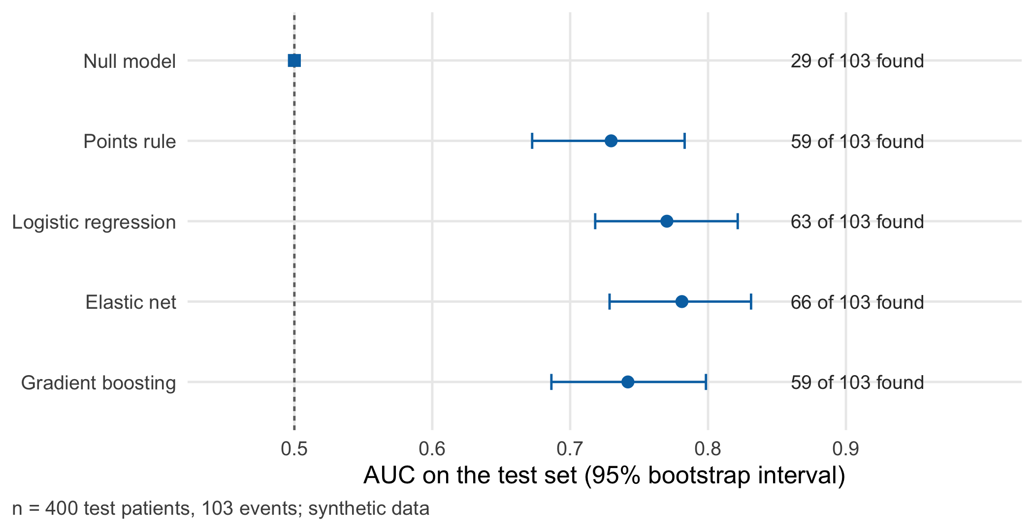
Two observations follow from Figure 5.1, which is computed in the lab. First, all models beat the null model by a wide margin, and the regression models rank patients somewhat better than the points rule. Second, the differences between regression, elastic net and boosting are small compared with the width of the intervals. With 400 test patients and about 100 events, an AUC difference of 0.02 cannot be distinguished from chance. The decision-relevant reading is the label: within the capacity of 120 patients, the candidates find between 59 and 66 of 103 future delirium cases. A handful of additional cases per 400 patients may matter — but only if the gain is real, holds in the next year’s patients, and is worth a data feed of 19 variables.
The most important assumption of this comparison is that the 400 test patients come from the same hospital, period and data-generating process as the development patients. Under this assumption a random hold-out set estimates how the model performs for similar patients; it says nothing about another hospital, a new protocol or next winter’s case mix.
A last point concerns honesty with the test set. If the team had compared ten models on the 400 test patients and reported the best, the winning number would be optimistic, because the test set would have been used for selection. In this chapter the choice of model family is fixed in advance and made on the inner cross-validation; the test set only confirms it.
Question for the workshop: In the test set the elastic net finds a few more cases than the rule and the regression, while boosting finds none more than the rule. Which additional evidence would you need before you accept the cost of a 19-variable data feed — and which of these questions could the hold-out test answer at all?
5.3 Lab
The lab runs in a fresh R session in well under a minute. It generates the cohort, splits it once, learns the preprocessing, tunes two models in the inner folds, compares all five candidates on the inner folds and finally predicts the test patients once.
5.3.1 Step 1 · Generate the synthetic cohort
Every value below is synthetic. The coefficients in the data-generating model are teaching assumptions, chosen to be clinically plausible in direction; they are not estimates from any study. Because the data are simulated we also know each patient’s true risk, which no real data set contains. We keep it for the counter-check in Chapter 6.
set.seed(2605)                                          # fixed start value for the whole lab
n <- 1200
id <- sprintf("P%04d", seq_len(n))                      # constant patient IDs, reused in B06

# Eight clinically motivated predictors
age <- pmin(101, 65 + round(rgamma(n, shape = 3.5, scale = 5)))           # years
cognitive_impairment <- rbinom(n, 1, plogis(-3.0 + 0.09 * (age - 65)))   # pre-existing, 0/1
asa <- as.integer(cut(rnorm(n, 0.03 * (age - 80), 1),                   # ASA class 1-4
                      c(-Inf, -1.7, 0, 1.25, Inf)))
haemoglobin <- round(rnorm(n, 12.0 - 0.02 * (age - 80), 1.6), 1)          # g/dL
sodium <- round(rnorm(n, 138.5, 4))                                       # mmol/L
n_medications <- rpois(n, 3 + 0.08 * (age - 65))                          # regular medicines
hours_to_surgery <- round(rgamma(n, shape = 2, scale = 14))               # hours from admission
sensory_impairment <- rbinom(n, 1, 0.3)                                   # vision or hearing, 0/1

# Eleven further routine variables; only CRP and albumin carry a weak signal
potassium <- round(rnorm(n, 4.2, 0.5), 1)        # mmol/L
creatinine <- round(rlnorm(n, log(1.0), 0.3), 2) # mg/dL
crp <- round(rlnorm(n, log(15), 1), 0)           # mg/L
leukocytes <- round(rlnorm(n, log(9), 0.3), 1)   # 10^9/L
glucose <- round(rlnorm(n, log(120), 0.25))      # mg/dL
albumin <- round(rnorm(n, 36, 5))                # g/L
bmi <- round(rnorm(n, 24, 4), 1)                 # kg/m^2
heart_rate <- round(rnorm(n, 85, 14))            # beats/min
systolic_bp <- round(rnorm(n, 140, 22))          # mmHg
temperature <- round(rnorm(n, 36.9, 0.4), 1)     # degrees C
spo2 <- pmin(100, round(rnorm(n, 95, 2.5)))      # %

# True linear predictor (assumption): includes a U-shaped sodium effect that no linear term captures
lp <- -1.6 + 0.065 * (age - 80) + 1.1 * cognitive_impairment + 0.35 * (asa - 2.7) -
  0.18 * (haemoglobin - 12) + 0.012 * ((sodium - 139)^2 - 16) + 0.09 * (n_medications - 4.5) +
  0.012 * (hours_to_surgery - 28) + 0.35 * sensory_impairment + 0.004 * (crp - 25) - 0.03 * (albumin - 36)
true_risk <- plogis(lp)
delirium <- rbinom(n, 1, true_risk)              # postoperative delirium within 5 days, 0/1

# Missing laboratory values (assumption: missing completely at random, see B03)
haemoglobin[sample(n, 70)] <- NA
sodium[sample(n, 45)] <- NA

cohort <- data.frame(id, age, cognitive_impairment, asa, haemoglobin, sodium, n_medications,
                     hours_to_surgery, sensory_impairment, potassium, creatinine, crp, leukocytes,
                     glucose, albumin, bmi, heart_rate, systolic_bp, temperature, spo2,
                     true_risk = round(true_risk, 4), delirium)
stopifnot(nrow(cohort) == 1200, !anyDuplicated(cohort$id), sum(cohort$delirium) == 320)
The cohort has 1,200 patients, 320 of whom develop delirium (26.7%).
5.3.2 Step 2 · Split once, by patient, and assign the inner folds
The split is made on patient IDs before any model sees the data. Each patient has one admission here; with repeated admissions the split would have to be made on the person, not the admission (Chapter 19).
test_ids <- sort(sample(cohort$id, 400))                        # independent test patients
cohort$split <- ifelse(cohort$id %in% test_ids, "test", "development")
dev_ids <- cohort$id[cohort$split == "development"]
inner_fold <- setNames(sample(rep(1:5, length.out = length(dev_ids))), dev_ids)
cohort$fold <- ifelse(cohort$split == "development", inner_fold[cohort$id], NA)  # 1-5; NA for test

dev <- cohort[cohort$split == "development", ]
test <- cohort[cohort$split == "test", ]
stopifnot(length(intersect(dev$id, test$id)) == 0,              # no patient in both sets
          nrow(dev) == 800, nrow(test) == 400,
          sum(dev$delirium) == 217, sum(test$delirium) == 103,
          all(table(dev$fold) == 160))
table(set = cohort$split, delirium = cohort$delirium)
#> delirium
#> set 0 1
#> development 583 217
#> test 297 1035.3.3 Step 3 · Learn the preprocessing from development data only
core <- c("age", "cognitive_impairment", "asa", "haemoglobin", "sodium", "n_medications",
          "hours_to_surgery", "sensory_impairment")
extra <- c("potassium", "creatinine", "crp", "leukocytes", "glucose", "albumin", "bmi",
           "heart_rate", "systolic_bp", "temperature", "spo2")
all_pred <- c(core, extra)

medians <- sapply(dev[all_pred], median, na.rm = TRUE)          # learned on development data
impute <- function(d, m) {                                      # applies stored medians, learns nothing
  for (v in names(m)) d[[v]][is.na(d[[v]])] <- m[[v]]
  d
}
dev_i <- impute(dev, medians)
test_i <- impute(test, medians)
stopifnot(!anyNA(dev_i[all_pred]), !anyNA(test_i[all_pred]))
medians[c("haemoglobin", "sodium")]
#> haemoglobin sodium
#> 11.9 139.0One simplification is deliberate and must be stated: the medians come from all 800 development patients, so inside the inner cross-validation the held-out fold has contributed a little to its own imputation. For a median this effect is negligible; for steps that learn more from the data, such as selecting predictors, it is not (see the box “Common mistake” below). A pipeline that refits every preprocessing step within each fold removes the issue.
5.3.4 Step 4 · Null model, points rule and logistic regression
auc <- function(p, y) {                       # rank formula (Mann-Whitney), equals the ROC area
  r <- rank(p); n1 <- as.double(sum(y)); n0 <- length(y) - n1
  (sum(r[y == 1]) - n1 * (n1 + 1) / 2) / (n1 * n0)
}
brier <- function(p, y) mean((p - y)^2)       # mean squared error of the predicted risk

rule_points <- function(d) (d$age >= 85) + d$cognitive_impairment + (d$asa >= 3)   # 0-3 points
fit_rule <- function(d) tapply(d$delirium, factor(rule_points(d), levels = 0:3), mean)
predict_rule <- function(tab, d) as.numeric(tab[as.character(rule_points(d))])

f_lr <- reformulate(core, response = "delirium")                # eight prespecified predictors, linear
fit_rule(dev_i)                                                 # observed risk per point (development)
#> 0 1 2 3
#> 0.1050420 0.1993671 0.3987342 0.75000005.3.5 Step 5 · Elastic net, tuned in the inner folds
cv.glmnet() (Friedman et al. 2010) runs the inner cross-validation for a sequence of shrinkage values λ. We pass our own fold vector so that every candidate sees the same folds, and repeat it for five values of the mixing parameter α (0 = ridge, 1 = lasso). The combination with the lowest cross-validated deviance is kept.
library(glmnet)
x_dev <- as.matrix(dev_i[all_pred]); x_test <- as.matrix(test_i[all_pred])
alphas <- c(0, 0.25, 0.5, 0.75, 1)
cv_fits <- lapply(alphas, function(a)
  cv.glmnet(x_dev, dev_i$delirium, family = "binomial", alpha = a,
            foldid = dev_i$fold, keep = TRUE))                    # keep = out-of-fold predictions
best <- which.min(sapply(cv_fits, function(cv) min(cv$cvm)))
en_cv <- cv_fits[[best]]
en_alpha <- alphas[best]; en_lambda <- en_cv$lambda.min
en_coef <- coef(en_cv, s = "lambda.min")
en_nonzero <- sum(en_coef[-1, 1] != 0)                          # predictors kept by the elastic net
c(alpha = en_alpha, lambda = round(en_lambda, 4), predictors_kept = en_nonzero)
#> alpha lambda predictors_kept
#> 0.2500 0.0244 15.00005.3.6 Step 6 · Gradient boosting, tuned in the inner folds
Depth, learning rate and minimum leaf size are fixed in advance; only the number of boosting rounds is tuned, with early stopping on the same five folds. With one thread and no subsampling the result is reproducible.
library(xgboost)
xgb_params <- list(objective = "binary:logistic", max_depth = 2, eta = 0.05,
                   min_child_weight = 5, eval_metric = "logloss", nthread = 1)
fold_index <- lapply(1:5, function(f) which(dev_i$fold == f))
xgb_cv <- xgb.cv(params = xgb_params, data = xgb.DMatrix(x_dev, label = dev_i$delirium),
                 nrounds = 1000, folds = fold_index, early_stopping_rounds = 30, verbose = 0)
xgb_rounds <- xgb_cv$early_stop$best_iteration
xgb_rounds
#> [1] 1105.3.7 Step 7 · Compare all candidates on the inner folds
All five candidates are now evaluated on the same inner folds of the development data. AUC and Brier score are computed per fold and averaged, so that the null model receives its correct AUC of 0.5. The test patients are still untouched.
oof <- data.frame(id = dev_i$id, fold = dev_i$fold, y = dev_i$delirium,
                  null = NA, rule = NA, lr = NA, en = NA, xgb = NA)
for (f in 1:5) {
  tr <- dev_i$fold != f; ho <- dev_i$fold == f                  # training folds and held-out fold
  oof$null[ho] <- mean(dev_i$delirium[tr])
  oof$rule[ho] <- predict_rule(fit_rule(dev_i[tr, ]), dev_i[ho, ])
  oof$lr[ho] <- predict(glm(f_lr, binomial, dev_i[tr, ]), dev_i[ho, ], type = "response")
  booster <- xgb.train(params = xgb_params, nrounds = xgb_rounds, verbose = 0,
                       data = xgb.DMatrix(x_dev[tr, ], label = dev_i$delirium[tr]))
  oof$xgb[ho] <- predict(booster, xgb.DMatrix(x_dev[ho, ]))
}
oof$en <- plogis(en_cv$fit.preval[, en_cv$index["min", 1]])     # out-of-fold, at the chosen lambda

models <- c(null = "Null model", rule = "Points rule", lr = "Logistic regression",
            en = "Elastic net", xgb = "Gradient boosting")
fold_mean <- function(metric, m) mean(sapply(1:5, function(f) {
  s <- oof$fold == f; metric(oof[[m]][s], oof$y[s]) }))
inner <- data.frame(model = models,
                    auc = sapply(names(models), function(m) fold_mean(auc, m)),
                    brier = sapply(names(models), function(m) fold_mean(brier, m)))
inner$auc[1] <- 0.5                                             # constant prediction: exactly 0.5
stopifnot(isTRUE(all.equal(fold_mean(auc, "null"), 0.5)))

# Prespecified choice of family: regression unless a flexible model is better by >= 0.02 AUC
gain_flex <- max(inner["en", "auc"], inner["xgb", "auc"]) - inner["lr", "auc"]
chosen <- if (gain_flex >= 0.02) "flexible model" else "logistic regression"
knitr::kable(inner, digits = 3, row.names = FALSE,
             col.names = c("Candidate", "AUC (inner CV)", "Brier score (inner CV)"),
caption = "Inner five-fold cross-validation on 800 synthetic development patients (217 with delirium); metrics averaged over folds.")| Candidate | AUC (inner CV) | Brier score (inner CV) |
|---|---|---|
| Null model | 0.500 | 0.198 |
| Points rule | 0.746 | 0.160 |
| Logistic regression | 0.775 | 0.150 |
| Elastic net | 0.773 | 0.152 |
| Gradient boosting | 0.757 | 0.157 |
On the development data the best flexible model differs from logistic regression by -0.002 in AUC, so the prespecified criterion selects logistic regression. The cross-validated values of the two tuned models are slightly optimistic, because the same folds served for tuning and for this comparison; nested cross-validation would remove that optimism.
5.3.8 Step 8 · Final fits and one look at the test set
lr_fit <- glm(f_lr, binomial, dev_i)
booster <- xgb.train(params = xgb_params, nrounds = xgb_rounds, verbose = 0,
                     data = xgb.DMatrix(x_dev, label = dev_i$delirium))
pred <- data.frame(id = test_i$id, y = test_i$delirium,
                   null = mean(dev_i$delirium),
                   rule = predict_rule(fit_rule(dev_i), test_i),
                   lr = predict(lr_fit, test_i, type = "response"),
                   en = as.numeric(predict(en_cv, newx = x_test, s = "lambda.min", type = "response")),
                   xgb = predict(booster, xgb.DMatrix(x_test)))
stopifnot(identical(pred$id, test$id))                          # same test patients for every candidate

# Paired bootstrap: resample test patients, recompute every AUC on the same resample
set.seed(5051)
boot <- replicate(2000, {
  i <- sample(nrow(pred), replace = TRUE)
  sapply(names(models)[-1], function(m) auc(pred[[m]][i], pred$y[i]))
})

# Decision-oriented reading: cases among the 120 highest-ranked patients (30% capacity).
# Ties (rule: four risk levels; null model: one) are broken in a fixed random order.
set.seed(5052)
tie_breaker <- runif(nrow(pred))
found_in_top <- function(p, y, k = 120) sum(y[order(-p, tie_breaker)[seq_len(k)]])

res <- data.frame(model = models,
                  auc = sapply(names(models), function(m) auc(pred[[m]], pred$y)),
                  lower = c(NA, apply(boot, 1, quantile, 0.025)),
                  upper = c(NA, apply(boot, 1, quantile, 0.975)),
                  brier = sapply(names(models), function(m) brier(pred[[m]], pred$y)),
                  found = sapply(names(models), function(m) found_in_top(pred[[m]], pred$y)),
                  predictors = c(0, 3, length(core), en_nonzero, length(all_pred)))
res$auc[1] <- 0.5
diff_xgb_lr <- quantile(boot["xgb", ] - boot["lr", ], c(0.025, 0.975))
diff_en_lr <- quantile(boot["en", ] - boot["lr", ], c(0.025, 0.975))
stopifnot(abs(res["lr", "auc"] - 0.770) < 0.002, abs(res["rule", "auc"] - 0.730) < 0.002,
          abs(res["en", "auc"] - 0.781) < 0.003, abs(res["xgb", "auc"] - 0.742) < 0.01,
          res["lr", "found"] == 63, sum(pred$y) == 103)
knitr::kable(res, digits = 3, row.names = FALSE,
             col.names = c("Candidate", "AUC", "2.5%", "97.5%", "Brier score",
                           "Cases in top 120", "Predictors used"),
caption = "Single evaluation on 400 synthetic test patients (103 with delirium). Interval: paired percentile bootstrap, 2,000 resamples of patients.")| Candidate | AUC | 2.5% | 97.5% | Brier score | Cases in top 120 | Predictors used |
|---|---|---|---|---|---|---|
| Null model | 0.500 | NA | NA | 0.191 | 29 | 0 |
| Points rule | 0.730 | 0.672 | 0.783 | 0.161 | 59 | 3 |
| Logistic regression | 0.770 | 0.718 | 0.822 | 0.157 | 63 | 8 |
| Elastic net | 0.781 | 0.729 | 0.831 | 0.152 | 66 | 15 |
| Gradient boosting | 0.742 | 0.686 | 0.798 | 0.163 | 59 | 19 |
The following code draws Figure 5.1 in the core reading from the objects res and pred.
library(ggplot2)
plot_df <- res
plot_df$model <- factor(plot_df$model, levels = rev(models))
plot_df$label <- paste0(plot_df$found, " of ", sum(pred$y), " found")
ggplot(plot_df, aes(x = auc, y = model)) +
  geom_vline(xintercept = 0.5, linetype = cdsr_linetypes[2], colour = cdsr_colours[["grey"]]) +
  geom_errorbar(aes(xmin = lower, xmax = upper), width = 0.2, orientation = "y",
                colour = cdsr_colours[["blue"]], na.rm = TRUE) +
  geom_point(aes(shape = model == "Null model"), size = 2.6, colour = cdsr_colours[["blue"]]) +
  geom_text(aes(x = 0.86, label = label), hjust = 0, size = 3.3, colour = "#333333") +
  scale_shape_manual(values = c(`FALSE` = cdsr_shapes[1], `TRUE` = cdsr_shapes[3]), guide = "none") +
  scale_x_continuous(limits = c(0.45, 1.0), breaks = seq(0.5, 0.9, 0.1)) +
  labs(x = "AUC on the test set (95% bootstrap interval)", y = NULL,
       caption = "n = 400 test patients, 103 events; synthetic data") +
  theme_cdsr()
The test results agree with the inner cross-validation in two respects: the regression ranks better than the rule, and no flexible model is clearly better than the regression. Boosting tends to rank slightly worse: the paired bootstrap interval for its AUC difference to the regression runs from -0.056 to 0.000. The elastic net tends to rank slightly better, with an interval from -0.001 to 0.024. Both intervals reach zero, and in cases found within the capacity the three models differ by at most 7 patients. Brier scores — the mean squared distance between predicted risk and outcome — tell the same story.
WarningCommon mistake
Learning from the test patients before the test. Typical forms are: choosing the ten predictors most strongly associated with delirium on the full data set and then cross-validating; standardising or imputing with statistics of all patients; trying several models on the test set and reporting the best. Each step lets information about the held-out outcomes leak into the model, and the reported performance becomes optimistic. PROBAST+AI therefore asks whether data leakage was avoided when data were split and whether all model development steps were repeated in each resampling round (Moons et al. 2025, model evaluation, signalling questions 4.5 and 4.6).
5.3.9 Step 9 · Export the teaching file
The cohort with its split and fold columns is written to data/b05-delirium-cohort.csv. Chapter 6 reads exactly this file, so both chapters use identical patients and identical test IDs.
write.csv(cohort, "../data/b05-delirium-cohort.csv", row.names = FALSE)
check <- read.csv("../data/b05-delirium-cohort.csv")
stopifnot(nrow(check) == 1200, sum(check$split == "test") == 400,
          identical(sort(check$id[check$split == "test"]), test_ids))
NoteOther implementation: Python/scikit-learn
Original implementation. scikit-learn (Pedregosa et al. 2011), stable release 1.9.1 (documentation checked November 2026): Pipeline, PredefinedSplit, GroupKFold, LogisticRegression.
Concrete advantage. A Pipeline of imputer, scaler and model, tuned with GridSearchCV, refits the preprocessing inside every inner fold and so removes the simplification of Step 3. GroupKFold keeps all admissions of a patient in one fold.
What must be identical. The input file data/b05-delirium-cohort.csv, its split column and its inner folds (imported with PredefinedSplit(test_fold = fold - 1), not regenerated), the unit (patient), the metrics and an agreed tolerance, for example ±0.005 in AUC. According to the scikit-learn user guide the penalty is divided by n·C, so glmnet’s λ corresponds to 1/(n·C) and α to l1_ratio (Friedman et al. 2010); glmnet standardises internally, scikit-learn only with a scaler in the pipeline. Elastic-net penalties need solver = "saga", the penalty argument is deprecated since version 1.8, and LogisticRegression is penalised by default (C = 1.0), so the unpenalised glm() of Step 4 corresponds to C = np.inf.
Status: conceptual comparison, not executed. No statement about speed is made.
5.4 Counter-check
Change one thing: the size of the development data. Keep the 400 test patients as they are, but develop the regression, the elastic net (with the mixing parameter chosen above) and the boosting model on a random subset of only 200 of the 800 development patients. Because a single subset is a single draw, repeat this 25 times.
Before you run the code, write down your prediction: Which candidate loses most discrimination? And in which direction does the calibration slope of each model move? The calibration slope is the coefficient obtained when the outcome is regressed on the logit of the predicted risk. A slope below 1 means that predictions are too extreme (high risks too high, low risks too low), which is typical of overfitting; a slope above 1 means that they are too cautious. Chapter 6 develops calibration in detail.
cal_slope <- function(p, y) unname(coef(glm(y ~ qlogis(p), family = binomial))[2])
one_small_run <- function() {
  small <- dev_i[dev_i$id %in% sample(dev_i$id, 200), ]        # 200 patients, inner folds kept
  x_small <- as.matrix(small[all_pred])
  p_lr <- predict(glm(f_lr, binomial, small), test_i, type = "response")
  en_s <- cv.glmnet(x_small, small$delirium, family = "binomial", alpha = en_alpha, foldid = small$fold)
  p_en <- as.numeric(predict(en_s, newx = x_test, s = "lambda.min", type = "response"))
  xgb_s <- xgb.cv(params = xgb_params, data = xgb.DMatrix(x_small, label = small$delirium),
                  nrounds = 1000, folds = lapply(1:5, function(f) which(small$fold == f)),
                  early_stopping_rounds = 30, verbose = 0)
  p_xgb <- predict(xgb.train(params = xgb_params, verbose = 0, nrounds = xgb_s$early_stop$best_iteration,
                             data = xgb.DMatrix(x_small, label = small$delirium)), xgb.DMatrix(x_test))
  c(events = sum(small$delirium),
    auc_lr = auc(p_lr, pred$y), auc_en = auc(p_en, pred$y), auc_xgb = auc(p_xgb, pred$y),
    slope_lr = cal_slope(p_lr, pred$y), slope_en = cal_slope(p_en, pred$y),
    slope_xgb = cal_slope(p_xgb, pred$y))
}
set.seed(5053)
runs <- t(replicate(25, one_small_run()))                       # 25 subsets x 7 results
q <- function(v) quantile(v, c(0.1, 0.5, 0.9))
counter <- data.frame(
  model = c("Logistic regression", "Elastic net", "Gradient boosting"),
  auc_800 = c(res["lr", "auc"], res["en", "auc"], res["xgb", "auc"]),
  auc_200 = sapply(c("auc_lr", "auc_en", "auc_xgb"), function(v) q(runs[, v])[2]),
  slope_800 = c(cal_slope(pred$lr, pred$y), cal_slope(pred$en, pred$y), cal_slope(pred$xgb, pred$y)),
  slope_200 = sapply(c("slope_lr", "slope_en", "slope_xgb"), function(v) q(runs[, v])[2]),
  slope_range = sapply(c("slope_lr", "slope_en", "slope_xgb"), function(v)
    paste(sprintf("%.2f", q(runs[, v])[c(1, 3)]), collapse = " to ")))
stopifnot(q(runs[, "slope_lr"])[3] < 1,                         # regression: too extreme in most runs
          q(runs[, "auc_xgb"])[2] < q(runs[, "auc_lr"])[2])
knitr::kable(counter, digits = 2, row.names = FALSE,
             col.names = c("Candidate", "AUC, 800 dev.", "AUC, 200 dev. (median)",
                           "Slope, 800 dev.", "Slope, 200 dev. (median)", "Slope, 10th to 90th percentile"),
caption = "Counter-check: development on 25 random subsets of 200 instead of 800 synthetic patients; evaluation always on the same 400 test patients.")| Candidate | AUC, 800 dev. | AUC, 200 dev. (median) | Slope, 800 dev. | Slope, 200 dev. (median) | Slope, 10th to 90th percentile |
|---|---|---|---|---|---|
| Logistic regression | 0.77 | 0.76 | 0.87 | 0.73 | 0.57 to 0.91 |
| Elastic net | 0.78 | 0.76 | 1.07 | 1.13 | 0.85 to 1.55 |
| Gradient boosting | 0.74 | 0.72 | 0.90 | 0.97 | 0.72 to 1.45 |
With 200 development patients the subsets contain a median of 54 events for eight prespecified predictors. Discrimination drops only modestly for the regression models and somewhat more for boosting, which has more to learn from fewer cases. The clearer change is in calibration. The unpenalised regression becomes systematically overconfident: its median slope is 0.73 and stays below 1 in at least 90% of the runs. The tuned models scatter in both directions, because the amount of shrinkage or the number of boosting rounds is itself estimated from few events — sometimes too much, sometimes too little. This is why the sample size of a prediction model is planned to limit overfitting and not only to estimate the AUC precisely (Riley et al. 2020). An AUC alone would have hidden the problem, which is the starting point of Chapter 6.
5.5 Consequences for patients and operations
Patients. The model decides who is offered prevention, so its errors fall on people: a patient ranked below the capacity line loses a chance of prevention. The points rule allocates care partly by age (85 or older), which needs a clinical justification and a check of how it treats younger patients with other risk factors. Whether errors fall unevenly on groups is a question for the test set, reported with denominators (Chapter 6, Chapter 21).
Operations. The rule needs three items the admitting clinician already knows; the regression eight values, two of them laboratory results with missing values; the flexible models a reliable feed of 19 variables, a documented imputation, a versioned model object and a plan for monitoring and updating (Chapter 20, Chapter 27). A gain of a few cases per 400 patients has to be weighed against these costs and against a feed that fails silently.
Regulation. As soon as the output is used to allocate care to individual patients, the intended purpose of the software has to be examined. If it qualifies as a medical device, Rule 11 in Annex VIII of the Medical Device Regulation classifies software that provides information used to take decisions with diagnostic or therapeutic purposes as class IIa or higher (European Parliament and Council of the European Union 2017); the guidance of the Medical Device Coordination Group (Medical Device Coordination Group 2025) — guidance, not binding law — describes how qualification is assessed. Whether an in-house pilot needs this assessment is a question for the local regulatory function (open; Chapter 22).
Data protection and security. Developing the model from routine data is a secondary use of health data and needs its own legal basis and documentation (Chapter 23, Chapter 26). The stored model and its preprocessing statistics are artefacts whose integrity has to be protected, because a changed median or coefficient changes every prediction (Chapter 24).
5.6 Look up and transfer
Reviewer question: “Which data informed the preprocessing, which the tuning, which the choice of model family and which the reported performance — and did any test patient contribute to the first three?” TRIPOD+AI asks authors to describe how the data were partitioned and to specify all model-building steps, including hyperparameter tuning and the method of internal validation (Collins et al. 2024, items 12a and 12c).
Self-test: A research group reports a random forest for delirium with an AUC of 0.86 from ten-fold cross-validation on all 600 patients of their hospital. Before the cross-validation they selected the ten predictors most strongly associated with delirium in the full data set. Which validation type is this, and what does the AUC of 0.86 estimate?
TipAnswer
It is internal validation by cross-validation, but with predictor selection outside the resampling loop. The selection has already seen the outcomes of every patient who is later held out, so the AUC of 0.86 is an optimistic estimate of the performance of the whole procedure. A correct estimate would repeat the selection inside each training fold (nested resampling) or confirm the final model on patients who played no part in development. Even then the result would describe new patients from the same hospital and period, not another hospital.
Annotated sources:
- Zou and Hastie (2005) introduces the elastic net, the penalty that mixes ridge and lasso and is tuned in Step 5.
- Friedman et al. (2010) describes the coordinate-descent algorithm and parameterisation of glmnet used in the lab.
- Chen and Guestrin (2016) describes the gradient-boosting system behind the flexible candidate.
- Christodoulou et al. (2019) is the systematic review showing no average benefit of machine learning over logistic regression in comparisons at low risk of bias.
- Varma and Simon (2006) shows that cross-validated error of a tuned classifier is biased and that nested cross-validation reduces the bias.
- Riley et al. (2020) supports the counter-check: sample size for prediction models must limit overfitting, not only ensure precise performance estimates.
- Moons et al. (2025) and Collins et al. (2024) provide the appraisal and reporting items cited for leakage, tuning and internal validation.
- Pedregosa et al. (2011) is the reference for the scikit-learn implementation in the comparison box.
- The Medical Device Regulation (European Parliament and Council of the European Union 2017) and MDCG 2019-11 Rev. 1 (Medical Device Coordination Group 2025) are the regulatory starting points for software that allocates care.
5.7 Further reading
- Chapter 6 — the same test patients, now with calibration, thresholds and consequences for two groups.
- Chapter 19 — what changes when the test patients come from another centre or a later period.
- Methods in R: Nested Cross-Validation — how to estimate the performance of a tuned procedure without a separate test set.
- Methods in R: Gradient Boosting — the tuning parameters fixed in Step 6 and their effect.
- CTTIR Courses, Course 4 · Cross-validation, nested CV, bootstrap .632+ — a full lab on resampling designs.
- CTTIR Courses, Course 4 · Regularisation: ridge, lasso, elastic net — practising the shrinkage path behind Step 5.
- CTTIR Courses, Course 2 · Logistic regression (binomial GLM) — the regression baseline in more depth.
- CTTIR Tutorials: XGBoost — a stand-alone tutorial on the boosting library used here.