n <- 600
age_levels <- c("18-29", "30-39", "40-49", "50-59", "60-69", "70-79", "80+")
districts  <- c("Northfield", "Eastbrook", "Southmoor", "Westvale")      # fictitious districts
injuries   <- c("acetabular fracture", "pelvic ring fracture", "femoral shaft fracture",
                "tibial plateau fracture", "ankle fracture")

registry <- data.frame(
  id       = sprintf("P%03d", 1:n),
  age_band = sample(age_levels, n, replace = TRUE, prob = c(.14, .12, .13, .15, .16, .16, .14)),
  sex      = sample(c("female", "male"), n, replace = TRUE),
  injury   = sample(injuries, n, replace = TRUE, prob = c(.15, .20, .20, .20, .25)),
  district = sample(districts, n, replace = TRUE, prob = c(.40, .30, .20, .10)),
  month    = sample(month.abb, n, replace = TRUE),
  icu      = rbinom(n, 1, 0.3)        # sensitive attribute: intensive care yes (1) / no (0)
)
# The rare group of the case: three young patients with an open pelvic fracture, all from Westvale
registry[1:3, c("injury", "district", "age_band")] <- list("open pelvic fracture", "Westvale", "18-29")
stopifnot(nrow(registry) == 600, sum(registry$injury == "open pelvic fracture") == 3)26 Secondary use and responsible open science
R. Heller · Date: 2025-12-14 · Last changed: 2026-11-09
26.1 Case and decision
A doctoral researcher has analysed an extract of 600 records from the fictitious trauma registry of a regional network. The journal asks for a data availability statement, and a co-author proposes to upload “the anonymised table” to a public repository: age band, sex, injury, home district, month of admission and whether the patient needed intensive care. Names and dates of birth have been removed. The registry’s data steward has to decide before submission what may be published openly, what can only be offered through controlled access and what stays inside the registry. One detail decides the case. Three young patients with an open pelvic fracture all live in the smallest district. In the proposed table each of them is alone in their row. Anyone who knows one of them – a neighbour, an employer, a journalist who covered the accident – can read off whether that person needed intensive care.
26.2 Core reading
26.2.1 Secondary use is a change of purpose
Registry and routine data were collected to treat patients or to assure the quality of care. Using them for a research question is secondary use, and legally it is a change of purpose. The General Data Protection Regulation (GDPR) states that further processing for scientific research is not considered incompatible with the original purpose, but only “in accordance with Article 89(1)”, which demands appropriate safeguards and, in particular, data minimisation (European Parliament and Council of the European Union 2016, Art. 5(1)(b) and 89(1)). Health data are a special category; their use for research needs a basis in Union or Member State law under Article 9(2)(j). In Germany this includes § 27 of the Federal Data Protection Act (Bundesdatenschutzgesetz, BDSG) (Federal Republic of Germany 2018) and, for health care providers that reuse their own care data, § 6 of the Health Data Use Act (Gesundheitsdatennutzungsgesetz, GDNG). The latter requires pseudonymisation, anonymisation as soon as the purpose allows, a concept of roles and rights, and logging of further processing (Federal Republic of Germany 2024). Which of these provisions applies to a particular registry, and whether state hospital law adds conditions, is a question for the institution’s data protection officer; a research label alone does not settle it. Ethics review is a separate step with its own body and its own questions (Chapter 21).
26.2.2 Openness in tiers
Open science does not mean that every file is public. The FAIR principles ask that data be findable, accessible, interoperable and reusable (Wilkinson et al. 2016); “accessible” can mean accessible under stated conditions. A practical plan therefore sorts every product of a project into tiers before the first upload (Table 26.1). Code, metadata and a synthetic example can usually be open. Aggregate results can be open after a disclosure check. Individual-level data go through controlled access. Raw images, video and the re-identification key do not leave the institution.
| Product | Example in the registry project | Access tier | Condition before release | Responsible role |
|---|---|---|---|---|
| Analysis code and package versions | R scripts, lock file | open, with licence | scan for embedded data, paths and passwords | principal investigator |
| Metadata and data dictionary | variable names, units, permitted values | open | rare category labels reviewed | data steward |
| Synthetic example data | same structure, values generated | open, marked synthetic | no record copied; limited usefulness stated | analyst and data steward |
| Aggregate results | tables, model coefficients | open after check | minimum cell size (here 5, an assumption); secondary suppression | analyst, checked by a second person |
| Pseudonymised individual-level data | registry extract | controlled access in a secure processing environment | legal basis, ethics vote, data use agreement, stated purpose | data access committee |
| Trained model | prediction model on registry data | controlled, or open after review | membership risk assessed (Chapter 25) | model owner |
| Raw images, video, free text | radiographs, clinical notes | not shared; analysis on site | – | controller (the institution) |
| Re-identification key | list linking pseudonyms to persons | never leaves the trusted third party | – | trusted third party |
26.2.3 Anonymity depends on the recipient
Removing names does not make a table anonymous. The GDPR asks whether a person can be identified by “all the means reasonably likely to be used”, explicitly including singling out (European Parliament and Council of the European Union 2016, recital 26). In September 2025 the Court of Justice of the European Union held, for the data protection regulation of EU institutions, that pseudonymised data are not personal data for every recipient in every case: identifiability has to be assessed for each person who processes the data. Data may be non-personal for a recipient only if that recipient cannot lift the pseudonymisation and cannot attribute the data by other means, such as cross-checking with other information (Court of Justice of the European Union 2025, paras 75–77). For the obligation to inform patients about recipients, identifiability is assessed from the controller’s point of view at the time of collection (para 111). Applying this reasoning to the GDPR is a professional interpretation, not the wording of the judgment; the parallel definitions make it plausible.
The key assumption of this chapter is that anonymity is a property of a dataset in a context, not of a list of variables. Whether a person can be singled out depends on who receives the data, what else that recipient knows and how small the groups are. Sweeney’s k-anonymity turns this into a checkable rule: every record must be indistinguishable from at least k − 1 others with respect to the quasi-identifiers, the attributes an outsider could know, such as age, sex, district or date (Sweeney 2002). Rare groups break the rule first. Rocher and colleagues estimated that 99.98% of Americans would be correctly re-identified in any dataset using 15 demographic attributes (published, Rocher et al. 2019). The European Health Data Space Regulation (EHDS) names the same residual risk for rare diseases, where small case numbers prevent full aggregation (European Parliament and Council of the European Union 2025, recital 92).
26.2.4 Reproducibility without exporting raw data
A reviewer wants to rerun the analysis; the patients want their records to stay where they are. Both are possible if the analysis travels to the data instead of the other way round. The code and a data dictionary are published. A synthetic example with the same structure lets anyone run the code from start to finish and see that it works. The real analysis runs in a secure processing environment, and only aggregate output that has passed a disclosure check leaves it. The reader can then reproduce every step and every table structure, and an authorised second analyst can reproduce every number. The paper should say which numbers belong to which group.
Question for the workshop: Take the data flow of your project (W5) or of the dashboard case (W7) and assign every product to a row of Table 26.1. Which group of patients in your data would be the first to be singled out, and which single change to the release would protect them?
26.3 Lab
The Lab builds the registry extract from the case, measures how identifiable its records are, and reduces the risk step by step. The extract is synthetic; the three records with an open pelvic fracture are placed deliberately.
An equivalence class is the set of records that share the same values on all quasi-identifiers. The function below returns, for each record, the size of its class; k is the smallest class size in the table.
class_size <- function(data, qi) {
  key <- do.call(paste, c(data[qi], sep = "|"))   # one key per combination of quasi-identifiers
  as.vector(table(key)[key])                       # size of the class each record belongs to
}

# Step 1: the table as proposed (five quasi-identifiers)
qi_raw <- c("age_band", "sex", "injury", "district", "month")
size_raw <- class_size(registry, qi_raw)

# Step 2: coarser age, two regions instead of four districts, month removed
release <- registry
release$age_group <- as.character(cut(match(release$age_band, age_levels), c(0, 3, 5, 7),
                                      labels = c("18-49", "50-69", "70+")))
release$region <- ifelse(release$district %in% c("Northfield", "Eastbrook"), "North-East", "South-West")
qi_gen <- c("age_group", "sex", "injury", "region")
size_gen <- class_size(release, qi_gen)

# Step 3: injuries grouped by body region
release$injury_group <- ifelse(release$injury %in% c("acetabular fracture", "pelvic ring fracture",
                                                     "open pelvic fracture"), "pelvis/acetabulum",
                        ifelse(release$injury == "femoral shaft fracture", "femur", "tibia/ankle"))
qi_grp <- c("age_group", "sex", "injury_group", "region")
size_grp <- class_size(release, qi_grp)

steps <- data.frame(
  step = c("1 as proposed", "2 age, region, no month", "3 + injury grouped"),
  k = c(min(size_raw), min(size_gen), min(size_grp)),
  unique_records = c(sum(size_raw == 1), sum(size_gen == 1), sum(size_grp == 1)),
  records_below_5 = c(sum(size_raw < 5), sum(size_gen < 5), sum(size_grp < 5))
)
steps
#> step k unique_records records_below_5
#> 1 1 as proposed 1 493 600
#> 2 2 age, region, no month 1 1 38
#> 3 3 + injury grouped 5 0 0stopifnot(steps$k[1] == 1, steps$k[2] == 1, steps$k[3] >= 5, steps$records_below_5[3] == 0)As proposed, 82.2% of the 600 records are unique on the five quasi-identifiers; k is 1. Coarser age and region and dropping the month reduce the records in classes smaller than 5 to 38, but k stays at 1: the rare patients are still alone. Only when injuries are grouped by body region does every class reach at least 5 records (Figure 26.1).
library(ggplot2)

cumulative <- function(sizes, label) {
  data.frame(release = label, size = 1:15, share = sapply(1:15, function(s) mean(sizes <= s)))
}
curve_df <- rbind(cumulative(size_raw, steps$step[1]), cumulative(size_gen, steps$step[2]),
                  cumulative(size_grp, steps$step[3]))
curve_df$release <- factor(curve_df$release, levels = steps$step)

ggplot(curve_df, aes(size, share, colour = release, linetype = release, shape = release)) +
  geom_vline(xintercept = 5, linetype = "22", colour = cdsr_colours[["grey"]]) +
  geom_line(linewidth = 0.8) +
  geom_point(size = 2) +
  scale_colour_manual(values = unname(cdsr_colours[c("orange", "blue", "green")])) +
  scale_linetype_manual(values = cdsr_linetypes[1:3]) +
  scale_shape_manual(values = cdsr_shapes[1:3]) +
  scale_y_continuous(labels = function(x) paste0(100 * x, "%"), limits = c(0, 1)) +
  scale_x_continuous(breaks = c(1, 5, 10, 15)) +
  labs(x = "Size of equivalence class (records)", y = "Cumulative share of records",
       colour = "Release", linetype = "Release", shape = "Release",
       caption = "Synthetic registry extract, n = 600 records; dashed line: k = 5.") +
  theme_cdsr() +
  guides(colour = guide_legend(ncol = 1))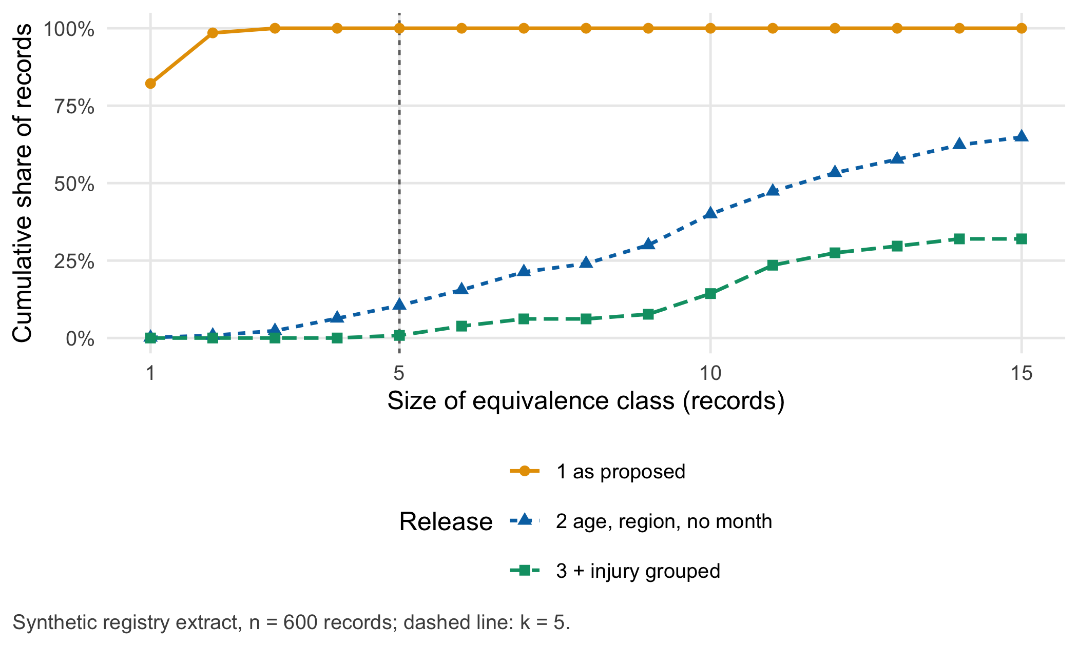
k-anonymity protects against singling out, not against learning a sensitive value. If all members of a class share the same intensive care status, knowing that a person belongs to the class reveals their status.
key_grp <- do.call(paste, c(release[qi_grp], sep = "|"))
homogeneous <- tapply(release$icu, key_grp, function(x) length(unique(x)) == 1)
n_classes <- length(homogeneous)
n_homogeneous <- sum(homogeneous)
homogeneous_sizes <- as.vector(table(key_grp)[names(homogeneous)[homogeneous]])
c(classes = n_classes, homogeneous = n_homogeneous)
#> classes homogeneous
#> 36 4homogeneous_sizes#> [1] 11 6 6 7stopifnot(n_classes == length(unique(key_grp)), all(homogeneous_sizes >= 5))In release 3, 4 of 36 classes are homogeneous for intensive care; they hold between 6 and 11 records each. For every member of these classes the open table would reveal the outcome, although k is at least 5. The sensitive column should therefore not be released at record level. The open release keeps the quasi-identifiers for description and offers the intensive care outcome only as an aggregate.
Aggregate tables have their own trap. The table below counts injuries by district, as a paper might print it. Cells with 1 to 4 records are suppressed (primary suppression). If a row or column then contains exactly one suppressed cell, the published total gives it away, so a second cell must be suppressed or the categories merged (secondary suppression).
counts <- table(injury = registry$injury, district = registry$district)
suppressed <- counts > 0 & counts < 5                     # primary suppression: 1-4 records
published <- ifelse(suppressed, "<5", as.character(counts))
published <- cbind(published, total = rowSums(counts))
published
#> Eastbrook Northfield Southmoor Westvale total
#> acetabular fracture "27" "37" "18" "10" "92"
#> ankle fracture "48" "73" "24" "14" "159"
#> femoral shaft fracture "41" "40" "25" "19" "125"
#> open pelvic fracture "0" "0" "0" "<5" "3"
#> pelvic ring fracture "34" "42" "23" "8" "107"
#> tibial plateau fracture "39" "37" "24" "14" "114"# A suppressed cell is recoverable if it is the only suppressed cell in a row or column with a published total
recoverable_rows <- rownames(counts)[rowSums(suppressed) == 1]
recoverable_cols <- colnames(counts)[colSums(suppressed) == 1]
list(rows = recoverable_rows, columns = recoverable_cols)#> $rows
#> [1] "open pelvic fracture"
#>
#> $columns
#> [1] "Westvale"stopifnot("open pelvic fracture" %in% recoverable_rows, "Westvale" %in% recoverable_cols,
counts["open pelvic fracture", "Westvale"] == 3)The row for open pelvic fractures shows three zeros, one suppressed cell and a total of 3: the suppression protects nobody. Merging the rare injury into the pelvic group removes the problem, at the price that the open table can no longer describe open pelvic fractures. That question moves to controlled access.
Finally the part of the plan that keeps the analysis reproducible. The data dictionary is published; a synthetic example with the same structure, but with values drawn independently for each column, lets anyone run the code.
dictionary <- list(age_band = age_levels, sex = c("female", "male"),
                   injury = c(injuries, "open pelvic fracture"), district = districts,
                   month = month.abb, icu = c(0, 1))

matches_dictionary <- function(data, dictionary) {
  identical(setdiff(names(data), "id"), names(dictionary)) &&
    all(mapply(function(values, allowed) all(values %in% allowed), data[names(dictionary)], dictionary))
}

# Open synthetic example: every column drawn independently from the permitted values
example <- data.frame(id = sprintf("SYN%03d", 1:50),
                      lapply(dictionary, function(allowed) sample(allowed, 50, replace = TRUE)))

# The same analysis code runs on both tables and returns the same structure
icu_by_injury <- function(data) aggregate(icu ~ injury, data = data, FUN = function(x) c(n = length(x), icu = sum(x)))

stopifnot(matches_dictionary(registry, dictionary), matches_dictionary(example, dictionary),
          identical(names(icu_by_injury(example)), names(icu_by_injury(registry))))
The example has no statistical value: every column was drawn on its own, so no association in it means anything. Its only purpose is that code, column names and permitted values can be tested in public while the registry stays in the secure environment.
26.4 Counter-check
A co-author wants to study seasonal patterns and asks to add the month of admission back to release 3. Predict first: what happens to k, and roughly what share of records will be in classes smaller than 5?
size_month <- class_size(release, c(qi_grp, "month"))
c(k = min(size_month), share_below_5 = round(mean(size_month < 5), 3))
#> k share_below_5
#> 1.000 0.852stopifnot(min(size_month) < 5, mean(size_month < 5) > 0.5)One extra attribute with twelve values divides every class by about twelve. k falls back to 1 and 85.2% of the records are in classes smaller than 5. The seasonal question is legitimate, but its answer belongs inside the secure environment, where the month can be used without being published, or in an aggregate table of admissions per month that does not carry the other quasi-identifiers. A second variation is worth predicting as well: raising the threshold from 5 to 10 never makes a release less safe, but every increase costs detail, and the rare groups pay first.
26.5 Consequences for patients and operations
Patients. The people most exposed are those with the rarest combination of features, and they are also the people whose cases are most often of scientific interest. A release plan that protects the average record but not the rare one fails exactly where it matters. Group harm is possible even when no individual is identified: a table that labels a small district by its intensive care rate can stigmatise its residents.
Ethics. Sharing has a benefit – independent checking, reuse, fewer redundant studies – and that benefit is a reason to share as much as can be shared safely, not a reason to share everything. The ethics committee should see the access matrix, not only the protocol (Chapter 21).
Data protection. The case changes the purpose of registry data, so the legal basis for research use, the safeguards under Article 89(1) GDPR and the recipients are documented before any transfer (Chapter 23). Pseudonymised individual records remain personal data for anyone who has, or could reasonably obtain, the means to re-identify them.
Regulation and governance: the EHDS in stages. The EHDS creates a common framework for secondary use of electronic health data. Its parts apply at different dates, so a statement such as “the EHDS requires” needs a date (Table 26.2). From 26 March 2029 health data access bodies decide on applications, issue data permits and provide access only through a secure processing environment; data are provided in anonymised form where the purpose allows, otherwise pseudonymised (European Parliament and Council of the European Union 2025, Art. 66 and 73). Users must not attempt re-identification and must make results public within 18 months, containing only anonymous data (Art. 61). Patients have a right to opt out of secondary use (Art. 71).
| Date | What applies | Relevance for the registry project |
|---|---|---|
| 5 March 2025 | publication in the Official Journal | text available; nothing applies yet |
| 25 March 2025 | entry into force (twentieth day after publication) | preparation by Member States begins |
| 26 March 2027 | general date of application; Member States notify their health data access bodies (Art. 55(6)); some provisions of Chapter IV | find out which body will be responsible for the network’s region |
| 26 March 2029 | Chapter IV on secondary use applies: data permits, secure processing environments, opt-out | registry data in the minimum categories (Art. 51) become available through access bodies |
| 26 March 2031 | Art. 51(1) points (b), (f), (g), (m), (p): determinants of health, genetic and other omics data, clinical trial and investigation data, research cohorts and surveys | cohort and questionnaire data of the project fall under the rules from this date |
| 26 March 2035 | Art. 75(5): third countries and international organisations as participants in HealthData@EU | relevant only for international partners |
Regional responsibility as an audit question. The EHDS lets each Member State designate one or more health data access bodies, with one acting as coordinator (European Parliament and Council of the European Union 2025, Art. 55(1)). Which body will be responsible for a regional trauma network in Germany is open at the time of writing; the audit path is the national implementing law and the list that Member States must make public. Data protection supervision in Germany is divided between federal and state authorities. For research projects whose controllers fall under several supervisory authorities, § 5 GDNG allows a joint notification that makes one authority the lead (Federal Republic of Germany 2024). The project should therefore record, for every partner, which supervisory authority, which ethics committee and, from 2027, which access body is responsible.
Security. A secure processing environment is only as good as its exit check. The EHDS requires access logs to be kept for at least one year and allows only non-personal data to be downloaded (European Parliament and Council of the European Union 2025, Art. 73). The disclosure check of the Lab is the human and technical step that makes “non-personal” true for each table.
26.6 Look up and transfer
Reviewer question: Which numbers in this paper can a reader reproduce from the published code and synthetic data, which require access to the controlled data, and is that split stated in the data availability statement?
Self-test: A gait study (Chapter 11) recorded video of 40 patients from a clinic for a rare neuromuscular disease and derived joint-angle time series. The authors want to publish the angle series together with age, sex and diagnosis subtype. Which product goes into which tier of Table 26.1, and which route to re-identification is the most likely?
TipAnswer
Code, data dictionary, a synthetic set of angle series and aggregate results (for example mean curves per subtype with the number of patients) can be open. The individual angle series belong in controlled access: a walking pattern can be characteristic of a person, and combined with age, sex and a rare subtype from a single clinic it may single them out. Raw video is not shared. The most likely route to re-identification is not the video file but the combination of a rare diagnosis subtype with demographic attributes and a known clinic, which is exactly the small-group problem of the Lab.
Annotated sources
- European Parliament and Council of the European Union (2016) – binding text for purpose limitation and research (Art. 5(1)(b), 6(4), 9(2)(j), 89(1)) and for identifiability and singling out (recital 26).
- Federal Republic of Germany (2018) and Federal Republic of Germany (2024) – German provisions for research use of personal and health data; § 6 GDNG for the reuse of care data by health care providers, § 5 GDNG for lead supervision of multi-state projects.
- European Parliament and Council of the European Union (2025) – binding text of the EHDS; used for the staged dates (Art. 105), access bodies (Art. 55), data minimisation (Art. 66), secure processing environments (Art. 73), duties of users (Art. 61), opt-out (Art. 71) and the residual risk for rare diseases (recital 92).
- Court of Justice of the European Union (2025) – judgment on pseudonymised data passed to a third party; source for the recipient-specific view of identifiability.
- Sweeney (2002) – original definition of k-anonymity and its limits.
- Rocher et al. (2019) – published estimate of how few demographic attributes suffice for re-identification.
- Wilkinson et al. (2016) – the FAIR principles, which separate “accessible” from “open”.
26.7 Further reading
- Chapter 23 – legal basis, recipients, pseudonymisation and deletion along the whole data flow.
- Chapter 3 – how rare combinations arise in the first place and how a teaching dataset is reduced.
- Chapter 4 – the reproducible R project that the synthetic example and the secure environment both run.
- Chapter 25 – membership disclosure, the model-level counterpart of the small-group problem.
- Scientometrics in R: Open Science Indicators – how open access, preprints and data availability statements are measured, and the limits of such indicators.
- Scientometrics in R: Reproducibility, RRIDs, and Badges – the gap between signalling reproducibility and achieving it.
- Scientometrics in R: Synthetic teaching records – a worked example of a synthetic fixture that states what it can and cannot establish.
- Methods in R: Writing a report – Reproducibility – what a reproducibility section of a paper should contain.